L04 · Hazards

Topic: pipelining · 59 pages

EECS 4340 · Lecture 4 — Pipelining Hazards

Show slide text

EECS 4340 — Lecture 4: Pipelining Hazards

Spring 2026 · Prof. Tanvir Ahmed Khan · https://courseworks2.columbia.edu/courses/237081

Slides developed in part by Profs. Austin, Brehob, Falsafi, Hill, Hoe, Lipasti, Martin, Roth, Shen, Smith, Sohi, Tyson, Vijaykumar, and Wenisch of Carnegie Mellon University, Purdue University, University of Michigan, University of Pennsylvania, and University of Wisconsin.

Announcements

Show slide text

Announcements

Lab #4 this Wednesday
- Please bring your computer
- Involve graded assignments
- Attendance is required and graded
Project #3
- Due: Milestone 18-Feb-26, full 25-Feb-26
Project #4
- Will be released today (16-Feb-26)
- Due: Project proposal 4-Mar-26, Milestone 1 11-Mar-26
- More details in the lab

https://courseworks2.columbia.edu/courses/237081

Readings

Show slide text

Readings

For today:

H & P Chapter C.1–C.4

For next week:

H & P Chapter C.5–C.7, 3.1–3.3, 3.10

Recap: Pipelining

Outline: Understanding the Execution Core

Show slide text

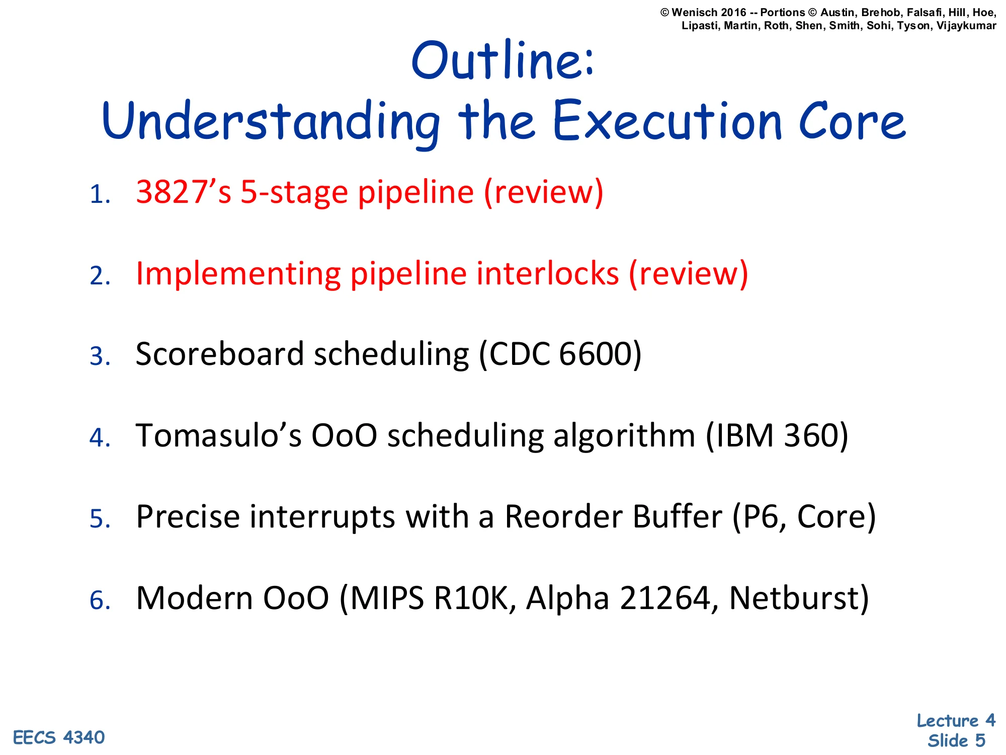
Outline: Understanding the Execution Core

3827’s 5-stage pipeline (review)
Implementing pipeline interlocks (review)
Scoreboard scheduling (CDC 6600)
Tomasulo’s OoO scheduling algorithm (IBM 360)
Precise interrupts with a Reorder Buffer (P6, Core)
Modern OoO (MIPS R10K, Alpha 21264, Netburst)

This is the roadmap for the execution-core arc of the course. Items 1–2 are review from the previous lecture: the 5-stage pipeline and the interlock logic that detects hazards. Today’s lecture (L04) focuses on those review items in depth — namely, how a pipelined datapath enforces program dependences when instructions in different stages need the same registers. The rest of the list previews future lectures: scoreboarding in the CDC 6600, Tomasulo’s algorithm in the IBM 360/91, the reorder buffer for precise interrupts in the Intel P6 microarchitecture, and modern out-of-order designs (MIPS R10K, Alpha 21264, Pentium 4 Netburst). The slide situates today’s hazard discussion as the foundation that all later out-of-order machinery is built on top of.

Pipelining

Show slide text

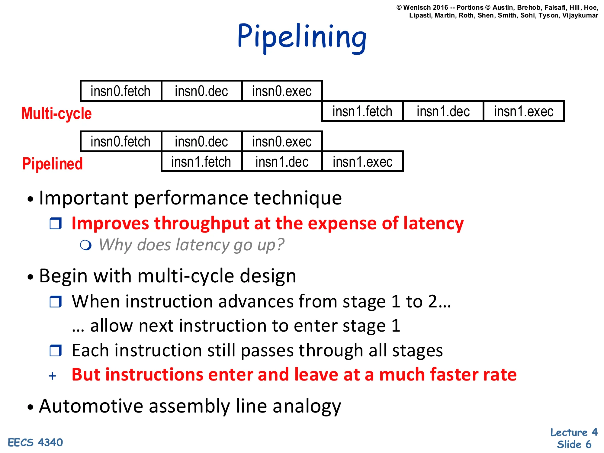
Pipelining

Multi-cycle: insn0.fetch | insn0.dec | insn0.exec then insn1.fetch | insn1.dec | insn1.exec (sequential).

Pipelined: insn0.fetch | insn0.dec | insn0.exec overlapped with insn1.fetch | insn1.dec | insn1.exec (one stage offset).

Important performance technique
- Improves throughput at the expense of latency
  - Why does latency go up?
Begin with multi-cycle design
- When instruction advances from stage 1 to 2… …allow next instruction to enter stage 1
- Each instruction still passes through all stages
- But instructions enter and leave at a much faster rate
Automotive assembly line analogy

Pipelining is the foundational throughput-improving trick covered in L03. The slide contrasts the multi-cycle datapath, where instruction $i+1$ cannot enter fetch until instruction $i$ has fully completed, with the pipelined datapath, where $i+1$ enters fetch as soon as $i$ vacates fetch. Both designs run each instruction through every stage, so the per-instruction latency does not shrink — in fact it grows slightly because pipeline registers add setup/clk-to-Q overhead between stages. What pipelining buys is throughput: instructions enter and leave at a rate of one per cycle (in the steady state), so total program time scales as $N + k - 1$ stages instead of $N \cdot k$ . The assembly-line analogy is the canonical mental model: each station works on a different car, and the whole line outputs one finished car per station-time. The italicised “why does latency go up?” is the lecturer’s prompt for the class — pipeline latches and clock-skew margins both eat into the per-stage time budget.

Time graphs

Show slide text

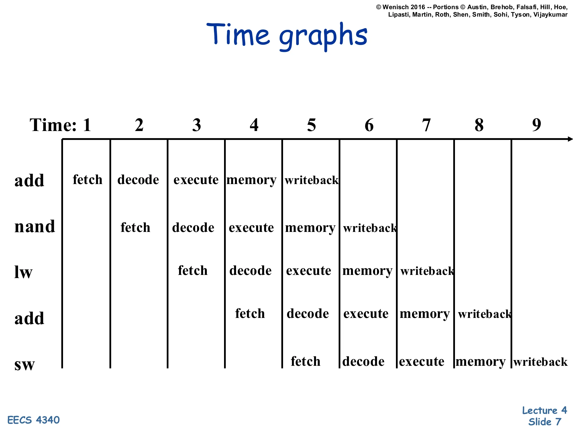
Time graphs

Pipeline diagram for a 5-stage pipeline (fetch / decode / execute / memory / writeback) over cycles 1–9.

Insn	1	2	3	4	5	6	7	8	9
add	F	D	E	M	W
nand		F	D	E	M	W
lw			F	D	E	M	W
add				F	D	E	M	W
sw					F	D	E	M	W

This is the standard “time-vs-instruction” diagram used throughout the lecture to reason about hazards. Each row is one dynamic instruction; each column is one clock cycle. A new instruction enters fetch every cycle, so after a four-cycle warm-up, the pipeline retires one instruction per cycle — an ideal IPC of 1. Because every column shows five different instructions occupying the five different stages simultaneously, two instructions that share a register can collide: e.g., the add in row 1 writes its destination in cycle 5 (W), but the nand in row 2 reads its source in cycle 3 (D). That two-cycle gap between when the producer commits and when the consumer needs the value is exactly the hazard window the rest of the lecture analyses. Subsequent slides will overlay stalls, forwarding paths, and squashes onto exactly this diagram.

5-stage datapath

Show slide text

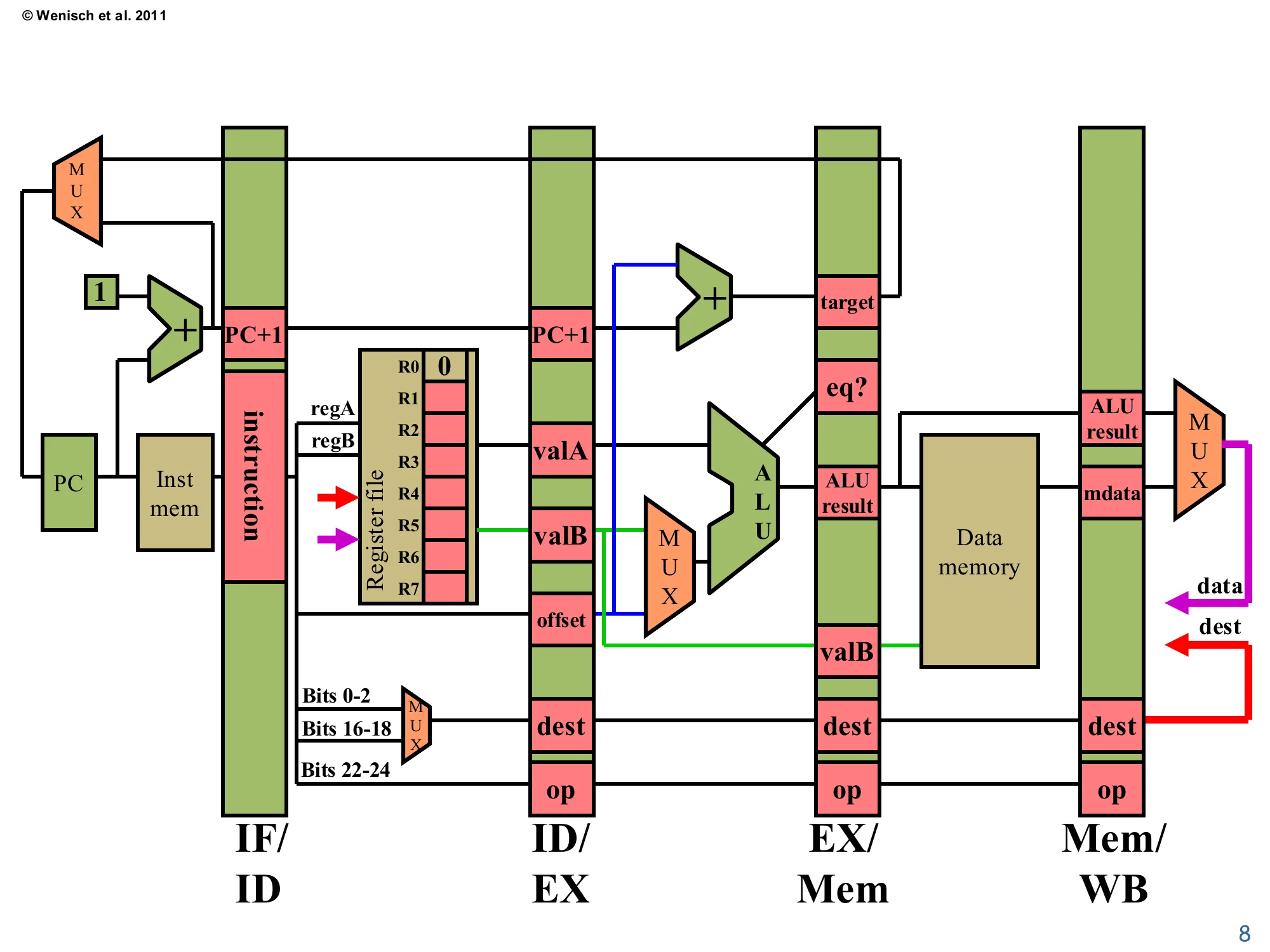
5-stage pipelined datapath (review from L03).

Stages, separated by pipeline registers IF/ID, ID/EX, EX/Mem, Mem/WB:

IF: PC → instruction memory; PC+1 adder; MUX selects PC+1 vs. branch target.
ID: instruction → register file (regA, regB) → valA, valB, offset; dest computed from instruction bits 0–2 / 16–18 / 22–24 via a MUX; control signals (op).
EX: ALU computes (valA op valB) or (valA + offset); branch target adder (PC+1 + offset); equality comparator (eq?).
Mem: data memory read/write using ALU result as address and valB as store data.
WB: MUX between ALU result (data) and memory data (mdata); written back to register file at dest. Writeback bus carries dest and data lines (red/purple).

This is the canonical 3827/MIPS-like five-stage datapath that the rest of the lecture annotates with hazard logic. Each green vertical band is a pipeline latch named for the stages it sits between (IF/ID, ID/EX, EX/Mem, Mem/WB); each pink slot inside a latch holds one field that survives into the next stage. Key fields to memorise: valA and valB are the register-file outputs read in ID, offset is the sign-extended immediate, dest is the architectural destination register chosen by a small MUX from instruction bits, and op carries the decoded opcode through every stage. The red “dest” and purple “data” wires looping back from Mem/WB into the register file are the writeback path: a register write completes in the WB stage, two cycles after the value is computed in EX. That gap is the source of every RAW data hazard discussed later — the consumer’s ID stage sees a stale register file before the producer’s WB has run.

Balancing Pipeline Stages

Show slide text

Balancing Pipeline Stages

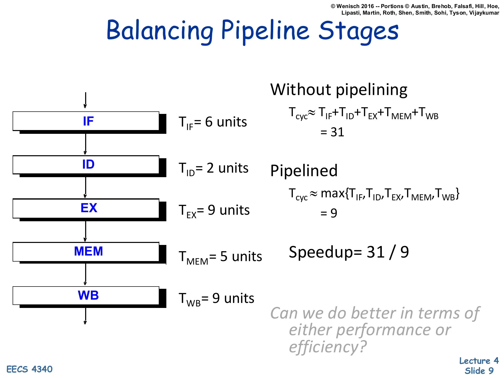
Stage delays: $T_{IF} = 6$ , $T_{ID} = 2$ , $T_{EX} = 9$ , $T_{MEM} = 5$ , $T_{WB} = 9$ (units).

Without pipelining: $T_{cyc} \approx T_{IF} + T_{ID} + T_{EX} + T_{MEM} + T_{WB} = 31$

Pipelined: $T_{cyc} \approx \max\{T_{IF}, T_{ID}, T_{EX}, T_{MEM}, T_{WB}\} = 9$

Speedup = 31 / 9

Can we do better in terms of either performance or efficiency?

This slide quantifies why pipelining helps and what limits it. Without pipelining, the cycle time has to absorb the full sum of stage delays, $\sum T_i = 31$ units, because every instruction traverses the whole datapath in one logical cycle. With pipelining, the cycle time is set by the slowest stage, $\max T_i = 9$ units (here the EX or WB stage). The speedup of $31/9 \approx 3.4\times$ is sub-linear because the stages are unbalanced — IF, ID, and MEM all finish in well under 9 units and waste the rest of the cycle waiting. The lecturer’s prompt at the bottom motivates the next slide: you can either merge a fast stage with a neighbour (raising $T_{cyc}$ but reducing pipeline depth) or subdivide the slow EX or WB stage into two pipeline stages (lowering $T_{cyc}$ at the cost of more hazards and more latches). This is one of the iron-law tradeoffs designers face.

Balancing Pipeline Stages (Trends)

Show slide text

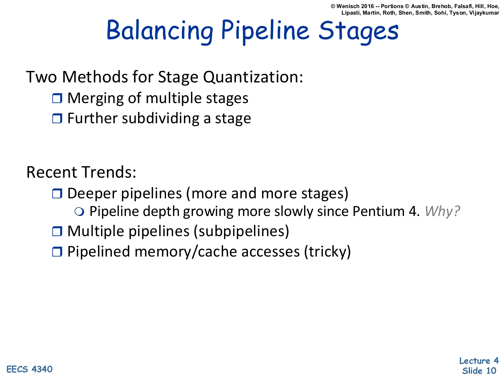
Balancing Pipeline Stages

Two Methods for Stage Quantization:

Merging of multiple stages
Further subdividing a stage

Recent Trends:

Deeper pipelines (more and more stages)
- Pipeline depth growing more slowly since Pentium 4. Why?
Multiple pipelines (subpipelines)
Pipelined memory/cache accesses (tricky)

The slide names the two re-balancing levers and then surveys what industry has actually done. Subdividing slow stages was pushed hardest by the Pentium 4 Netburst architecture, which went to 20+ stages to chase higher clock frequencies. Why did the trend slow after Pentium 4? Two reasons that the lecturer expects students to recall: (1) deeper pipelines amplify the cost of every branch misprediction and every RAW stall, eroding IPC faster than $f$ rises, and (2) the dynamic-power wall ( $P \propto C V^2 f$ , with $V$ scaled by DVFS limits) capped achievable frequencies regardless of pipeline depth. Modern x86 cores have settled near 14–16 stages and instead chase performance through wider issue (multiple parallel pipelines per cycle) and aggressive cache pipelining. The “tricky” caveat on cache pipelining foreshadows L05–L06: a pipelined cache must support multiple outstanding misses without violating the memory-ordering model.

Pipelining Hazards

The Cost of Deeper Pipelines

Show slide text

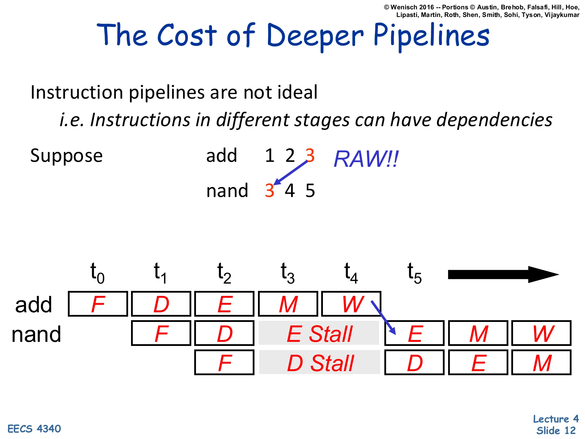
The Cost of Deeper Pipelines

Instruction pipelines are not ideal i.e. Instructions in different stages can have dependencies

Suppose: add 1 2 3 writes R3, then nand 3 4 5 reads R3 → RAW!!

Pipeline diagram:

Insn	t0	t1	t2	t3	t4	t5	t6	t7
add	F	D	E	M	W
nand		F	D	E Stall		E	M	W
			F	D Stall		D	E	M

The add writes R3 at t4 (W), but nand would read R3 at t2 (D) — must stall.

This slide opens the central problem of the lecture: even an ideal pipeline cannot run at one instruction per cycle because of inter-instruction dependencies. The example is a textbook read-after-write hazard (“RAW!!” in the slide). The producer add 1 2 3 writes architectural register R3 in its writeback stage at $t_4$ . The consumer nand 3 4 5 would read R3 in its decode stage at $t_2$ — two cycles too early, getting the stale value still sitting in the register file. The grey “E Stall / D Stall” boxes show one fix: freeze the consumer’s decode stage and bubble the execute stage with NOPs until the producer’s W has updated the register file. Each stalled cycle costs IPC, which is what motivates the rest of the lecture’s solutions (avoidance via NOPs, dynamic detect-and-stall, and detect-and-forward). The instruction below nand cascades the stall through fetch, mirroring how a single hazard ripples backwards through the front end.

Types of Dependencies and Hazards

Show slide text

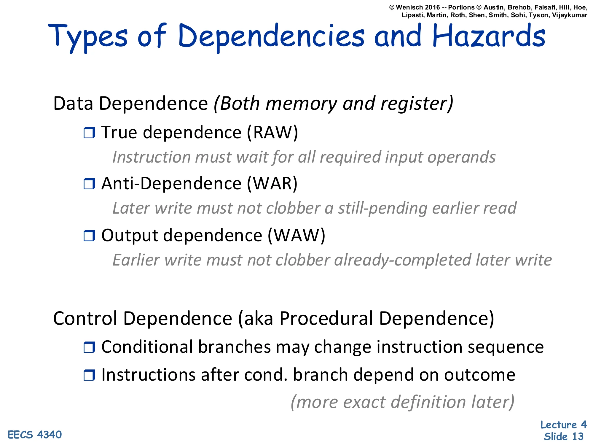
Types of Dependencies and Hazards

Data Dependence (Both memory and register)

True dependence (RAW)
- Instruction must wait for all required input operands
Anti-Dependence (WAR)
- Later write must not clobber a still-pending earlier read
Output dependence (WAW)
- Earlier write must not clobber already-completed later write

Control Dependence (aka Procedural Dependence)

Conditional branches may change instruction sequence
Instructions after cond. branch depend on outcome
- (more exact definition later)

This is the canonical taxonomy that every hazard discussion in this course will refer back to. Data dependences come in three flavours, named for the order of the read (R) and write (W) operations. RAW is the true dependence: the consumer literally needs the value the producer is about to write — no clever renaming can remove it. WAR and WAW are false (or name) dependences: they only exist because two instructions happen to use the same architectural register name; if the hardware renames the destinations to physical registers, the conflict disappears. The slide notes that all three apply equally to memory locations as to registers — this matters in L07 when we discuss memory disambiguation. Control dependence is a separate category: even with all data dependences satisfied, a branch can change which instructions should execute at all, so the front end can’t safely fetch past an unresolved branch without speculation.

Terminology

Show slide text

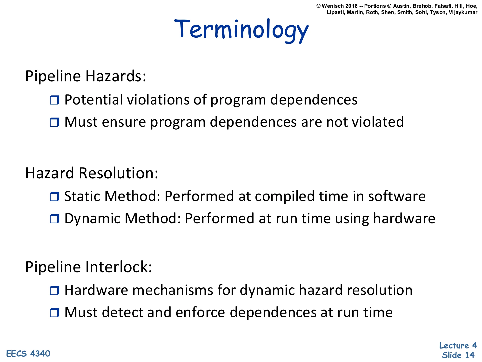
Terminology

Pipeline Hazards:

Potential violations of program dependences
Must ensure program dependences are not violated

Hazard Resolution:

Static Method: Performed at compiled time in software
Dynamic Method: Performed at run time using hardware

Pipeline Interlock:

Hardware mechanisms for dynamic hazard resolution
Must detect and enforce dependences at run time

The slide draws a careful distinction the rest of the lecture relies on. A dependence is a property of the program — instruction $j$ uses a value produced by instruction $i$ — and it is fixed by the source code regardless of hardware. A hazard is a property of the implementation: a situation where the pipeline could violate the dependence if it didn’t take corrective action. Three or more programs with the same dependences can therefore have different hazards on different machines. Hazard resolution picks who fixes the problem. Static methods (NOP insertion, instruction scheduling) push the work to the compiler and bake it into the binary. Dynamic methods use pipeline interlocks — comparators and stall logic — to detect dependences at runtime and slow the pipeline as needed. The same vocabulary recurs in scoreboarding and Tomasulo later in the term, where interlocks are generalised to arbitrary functional-unit latencies and out-of-order issue.

Necessary Conditions for Data Hazards

Show slide text

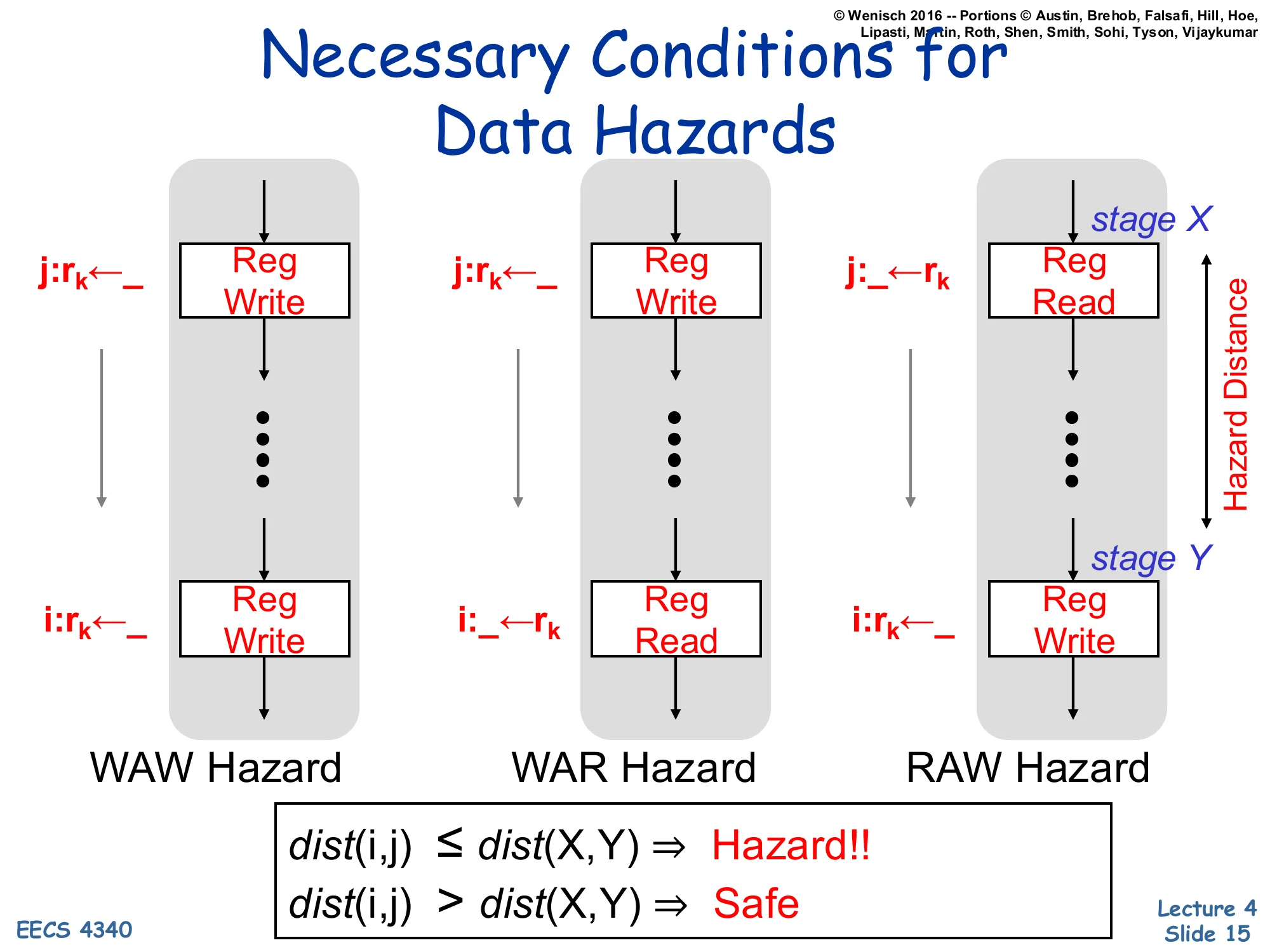
Necessary Conditions for Data Hazards

For each hazard type, compare instructions $i$ (older) and $j$ (younger) accessing register $r_k$ :

WAW Hazard: $j: r_k \leftarrow \_$ (Reg Write at stage X) … $i: r_k \leftarrow \_$ (Reg Write at stage Y)
WAR Hazard: $j: r_k \leftarrow \_$ (Reg Write at stage X) … $i: \_ \leftarrow r_k$ (Reg Read at stage Y)
RAW Hazard: $j: \_ \leftarrow r_k$ (Reg Read at stage X) … $i: r_k \leftarrow \_$ (Reg Write at stage Y)

Hazard distance = distance between stage X (where younger op happens) and stage Y (where older op happens).

$dist(i,j) \le dist(X, Y) \Rightarrow \text{Hazard!!}$ $dist(i,j) > dist(X, Y) \Rightarrow \text{Safe}$

This slide gives the formal condition under which a data hazard can actually occur in a given pipeline. The intuition: a hazard exists only if the younger instruction’s access stage (X) reaches it before the older instruction has finished its access stage (Y). For RAW in the standard 5-stage pipeline, the consumer reads in ID (stage 2) and the producer writes in WB (stage 5), so $dist(X,Y) = 3$ : any consumer fewer than 3 instructions behind the producer hits the hazard. The same framework applies to WAR and WAW — but in an in-order pipeline that always reads in ID and writes in WB, WAR and WAW are never triggered (the older instruction always reaches its access stage first). They become real concerns only once you allow out-of-order execution or multi-cycle functional units, which is why the rest of the course revisits this condition in scoreboarding and Tomasulo. The decision rule at the bottom — comparing $dist(i,j)$ to $dist(X,Y)$ — is the litmus test you’d apply on an exam to decide whether a code snippet on a given pipeline contains an actual hazard.

Handling Data Hazards

Show slide text

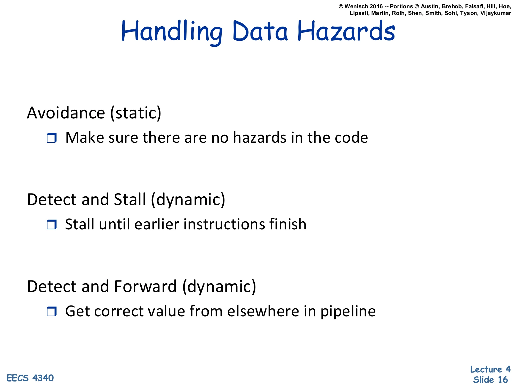
Handling Data Hazards

Avoidance (static)

Make sure there are no hazards in the code

Detect and Stall (dynamic)

Stall until earlier instructions finish

Detect and Forward (dynamic)

Get correct value from elsewhere in pipeline

This slide is the agenda card for the next ~25 slides: three families of solutions to RAW hazards in an in-order pipeline. Avoidance is purely software: insert enough NOPs (or schedule independent instructions) so the dependent consumer is far enough behind the producer that no hazard ever arises. Detect and stall is the simplest hardware solution: a comparator in ID checks the source registers against destinations of in-flight instructions; on a match it freezes IF/ID and feeds bubbles into EX until the producer drains. Detect and forward (a.k.a. bypassing) is the most aggressive hardware solution: when the producer’s result is available in EX/Mem or Mem/WB, route it directly into the consumer’s ALU inputs, avoiding the stall entirely. The lecture will walk through each in order, weighing the implementation cost against the CPI impact. All three are still used in modern CPUs — even out-of-order processors rely on forwarding networks to deliver results between back-to-back dependent micro-ops.

Handling Data Hazards: Avoidance

Show slide text

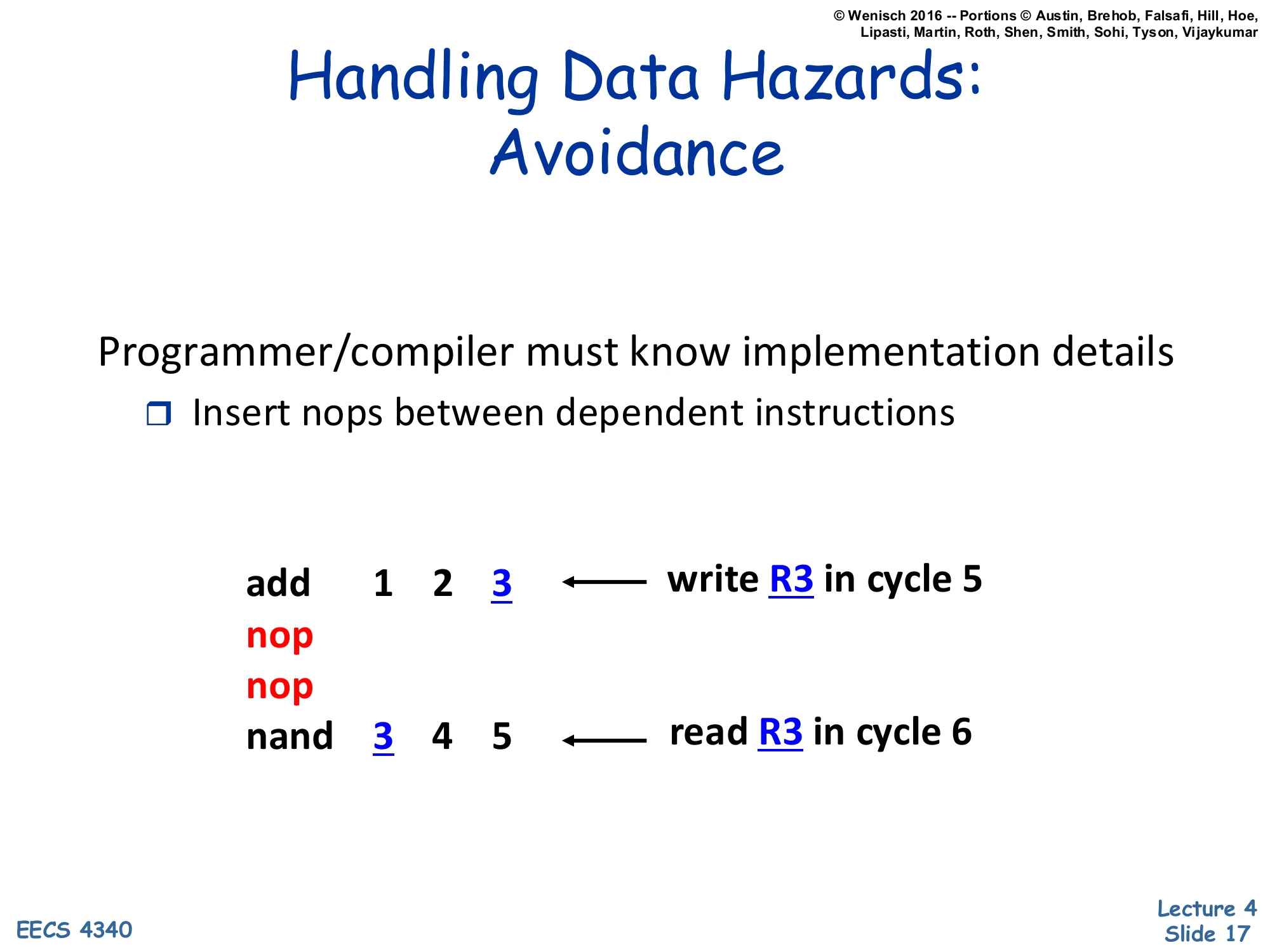
Handling Data Hazards: Avoidance

Programmer/compiler must know implementation details

Insert nops between dependent instructions

add  1 2 3   ← write R3 in cycle 5
nop
nop
nand 3 4 5   ← read R3 in cycle 6

The static avoidance scheme makes the compiler responsible for hazards. In the example, the producer add 1 2 3 writes R3 in its WB stage during cycle 5; the consumer nand 3 4 5 is now scheduled two NOPs later, so its ID stage falls in cycle 6 — exactly one cycle after the writeback completes (assuming the register file supports write-then-read in the same cycle, which most designs do). Notice that the compiler must know the exact hazard distance for the target microarchitecture: a deeper pipeline would need three NOPs, a forwarding-equipped pipeline none. That coupling is the central problem with avoidance and is the topic of the next slide. The technique is not extinct, though: VLIW and DSP architectures still expose hazards to the compiler, and even mainstream ISAs such as MIPS retained a load-delay slot (one mandatory NOP after a load) for binary-compatibility reasons in early implementations.

Problems with Avoidance

Show slide text

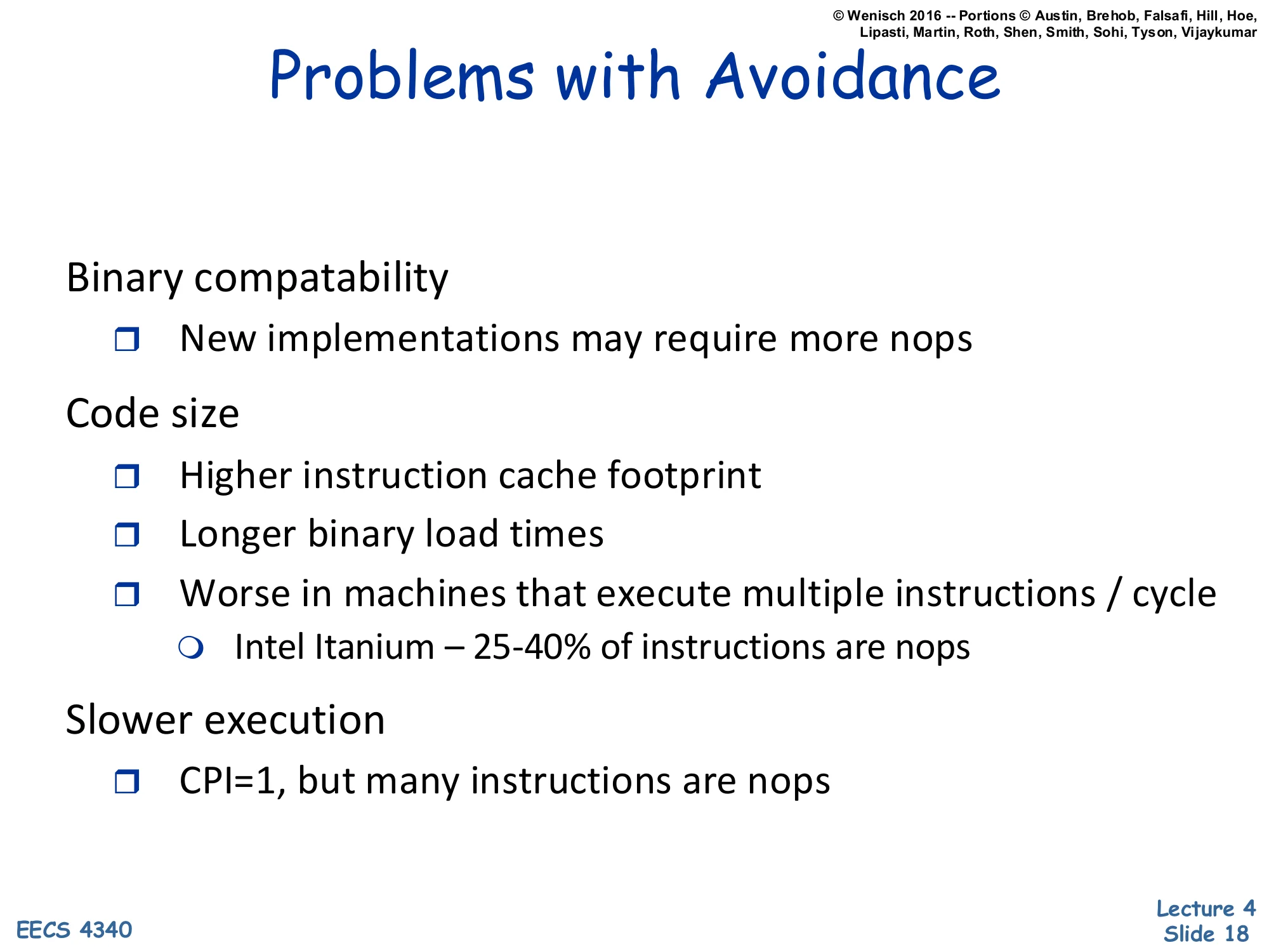
Problems with Avoidance

Binary compatability

New implementations may require more nops

Code size

Higher instruction cache footprint
Longer binary load times
Worse in machines that execute multiple instructions / cycle
- Intel Itanium – 25–40% of instructions are nops

Slower execution

CPI=1, but many instructions are nops

This slide catalogues why avoidance lost out to dynamic interlocks for general-purpose CPUs. Binary compatibility is the showstopper: a binary scheduled for an older, shallower pipeline will run incorrectly on a deeper successor unless the new chip also implements interlocks as a backstop. Code size explodes when NOPs are inserted everywhere — the lecturer cites Intel’s Itanium VLIW (EPIC) processor, where 25–40% of instruction slots in real binaries were unused and filled with NOPs, severely hurting instruction-cache footprint. The third bullet is subtle: even if the CPI is technically 1.0 (every cycle retires one instruction), many of those instructions are NOPs that do no useful work, so the effective CPI for real work is higher. The Itanium experience is widely cited as evidence that the compiler cannot reliably schedule around all hazards in real workloads — memory latencies in particular are too unpredictable. Modern x86 and ARM cores do hazard resolution dynamically in hardware for exactly these reasons.

Handling Data Hazards: Detect & Stall

Show slide text

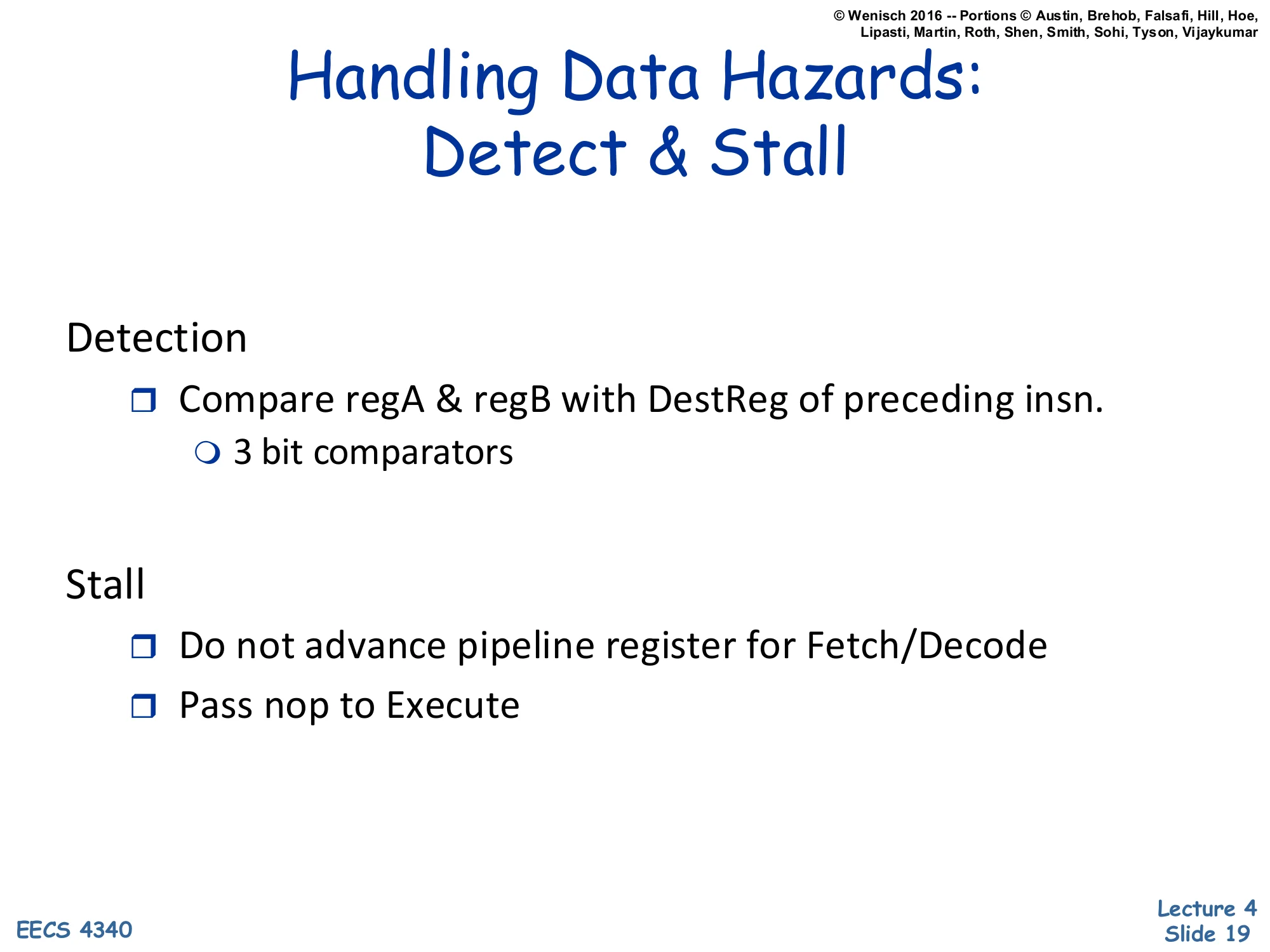
Handling Data Hazards: Detect & Stall

Detection

Compare regA & regB with DestReg of preceding insn.
- 3 bit comparators

Stall

Do not advance pipeline register for Fetch/Decode
Pass nop to Execute

This is the simplest dynamic hazard-resolution scheme. Detection happens in ID: each cycle, the decode logic compares the two source-register fields (regA, regB) of the instruction currently in IF/ID against the destination register field of every instruction still ahead of it in ID/EX, EX/Mem, and Mem/WB. Because the example ISA has 8 architectural registers, each comparator needs only 3 bits of equality logic — cheap silicon. Stall happens by clock-gating the IF/ID and PC registers (so they hold their current values for another cycle) and simultaneously injecting a NOP into the ID/EX latch (so EX has no useful work to do this cycle). The result is a one-cycle bubble that propagates down the pipe; on the next cycle, detection re-runs and either stalls again or releases. Two important properties: the scheme costs no extra cycles when there is no hazard (zero overhead in the common case), and it always makes forwarding correctness easier later — once detect-and-stall works, forwarding is just “detect and provide the value early instead of stalling.”

5-stage datapath (relabelled)

Show slide text

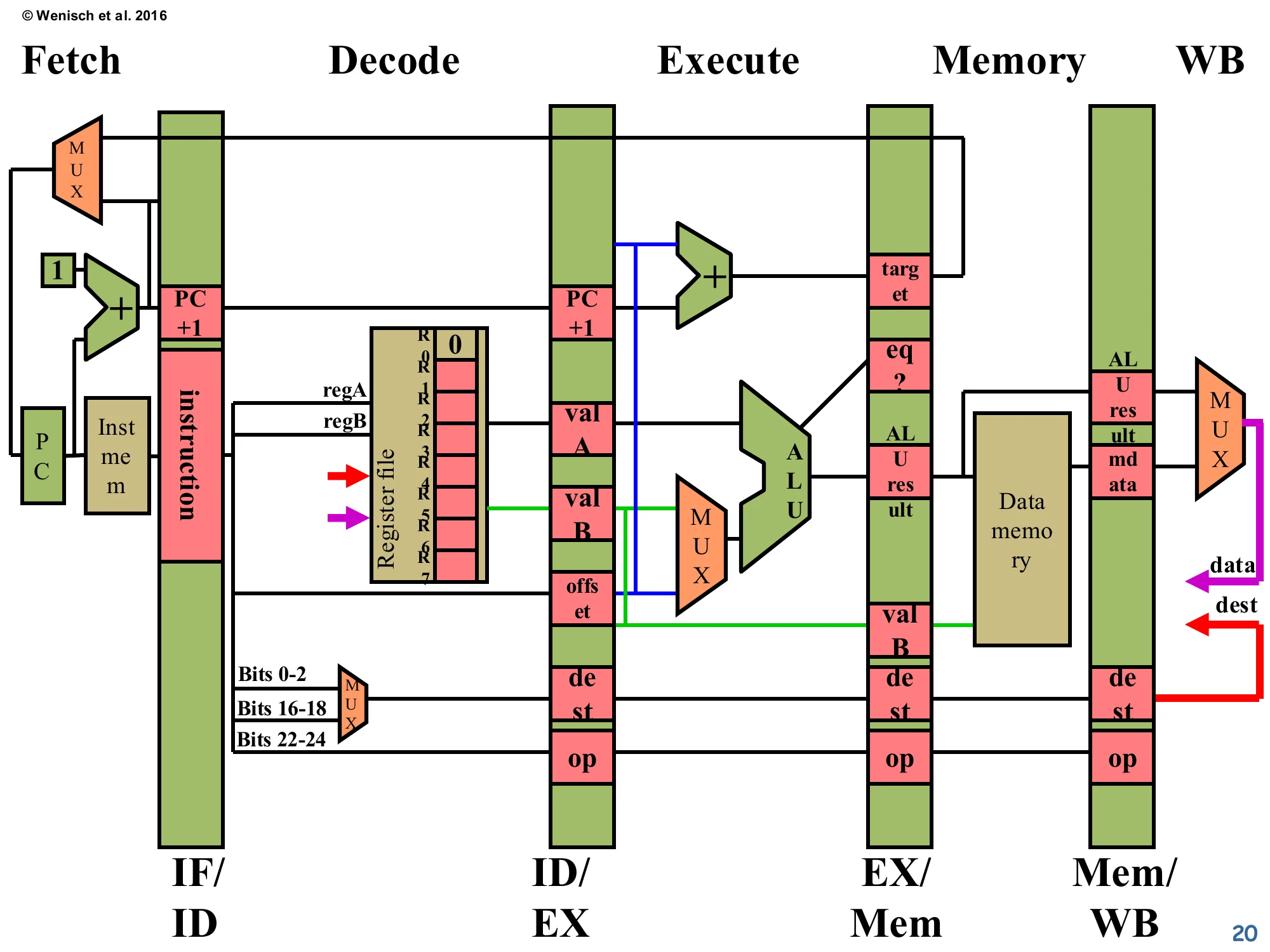
5-stage datapath (Wenisch 2016 redraw with stage names)

Stages: Fetch · Decode · Execute · Memory · WB, separated by IF/ID, ID/EX, EX/Mem, Mem/WB pipeline latches.

Same components as the L03 datapath: PC, instruction memory, register file (R0–R7), ALU, branch-target adder, equality comparator, data memory, writeback MUX between ALU result and mdata. The dest field flows from the decode-stage MUX (selecting bits 0–2, 16–18, or 22–24 of the instruction) through every latch back to the register file’s write port.

This slide is the same datapath diagram from page 8, redrawn with the more conventional stage labels (“Fetch / Decode / Execute / Memory / WB” written across the top instead of just IF/ID/EX/M/WB on the latches). The lecturer reuses this exact figure as the canvas for the next dozen slides, which animate a hazard scenario cycle-by-cycle. Fixing the layout in your head now pays off: you should be able to point to where valA, valB, dest, and op live in each pipeline latch, where the writeback bus (red dest and purple data wires) loops back into the register file’s write port, and where the branch-target adder sits in EX. Every later slide annotates this skeleton with comparators, stalls, NOP injections, and forwarding muxes — the structure of the underlying datapath never changes.

Datapath with Hazard Comparators

Show slide text

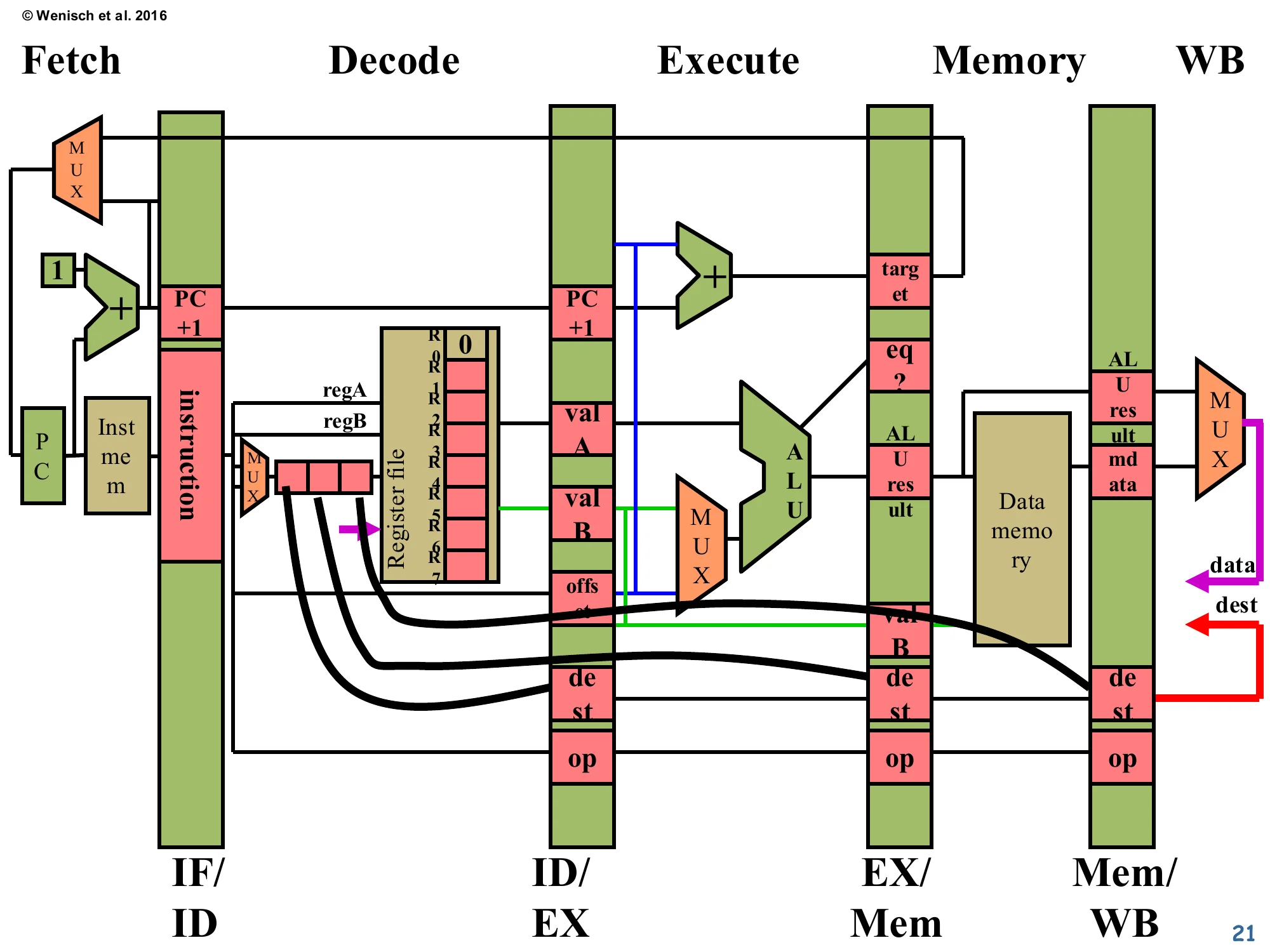
Datapath with Hazard Comparators

The redrawn datapath now shows a 3-element queue of dest fields fanning out from the decode stage. The black wires sweep right and connect each in-flight dest register (in ID/EX, EX/Mem, Mem/WB) back to a fresh hazard-detection MUX added on the left side of decode. This is the physical realisation of the comparator network described on the previous slide: the IF/ID instruction’s two source fields will be compared against all three pending destinations in parallel, every cycle.

This slide makes the comparator network concrete by overlaying it on the datapath. Three black arcs run from the dest slots in ID/EX, EX/Mem, and Mem/WB back to a small MUX/comparator block at the left of decode. The new MUX on the left is where the comparators look up the three potentially-conflicting destinations and, on any match, raise a single “hazard-detected” signal. Three pipeline stages × two source registers per consumer = six comparators total. Each comparator is only 3 bits wide for this 8-register ISA, so the area cost is trivial. The wires are long, however — they cross most of the datapath horizontally — and on real silicon their RC delay is what eventually limits how aggressively forwarding can be implemented. This is the foundation that the next several slides will exercise on a worked example: producer add 1 2 3 followed by consumer nand 3 4 5.

End of Cycle 1

Show slide text

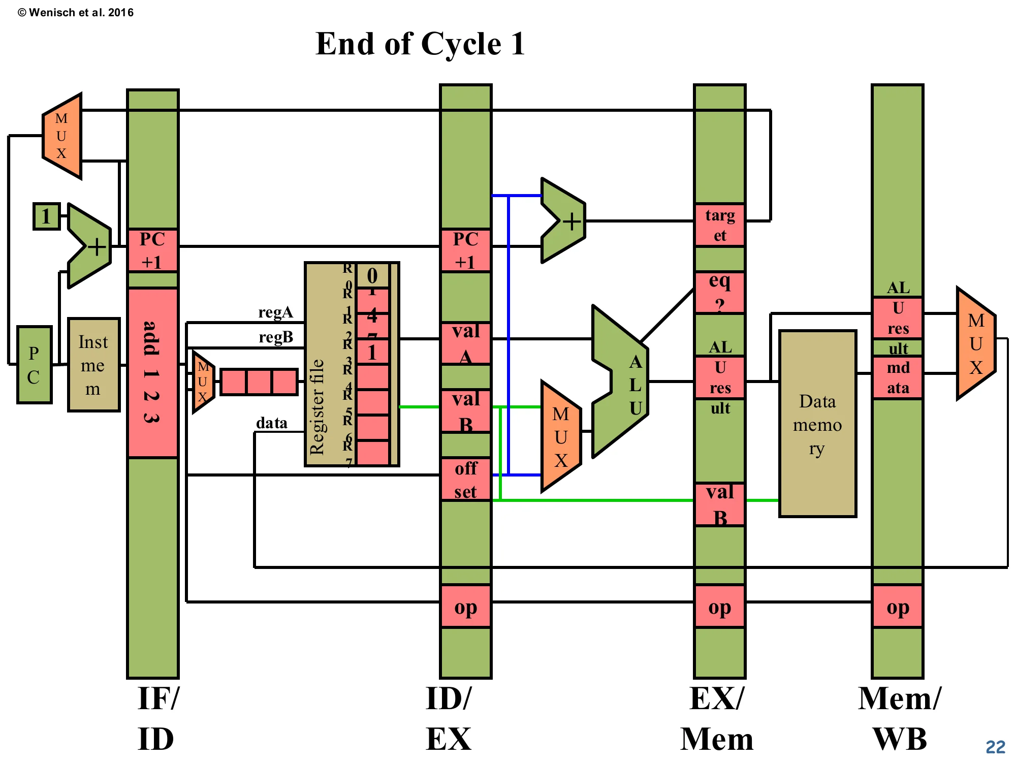
End of Cycle 1

IF/ID latch holds add 1 2 3. Register file shows initial contents (R0=0, R1=4, R2=7, others 0). The add has been fetched but not yet decoded — its source and destination fields are still in the IF/ID register awaiting the comparator network.

The lecturer steps through a five-cycle pipeline trace to show detect-and-stall in action. At end-of-cycle-1, only the producer instruction add 1 2 3 has been fetched. Its encoding (“add 1 2 3” written across the IF/ID latch) means “R3 ← R1 + R2” — read R1 and R2, write R3. The register file pre-contents R1=4, R2=7 are visible because the diagram will track real values flowing through the datapath as the example runs. No hazard yet — there’s only one instruction in flight, nothing to compare against. The pipeline is one cycle into warm-up.

End of Cycle 2

Show slide text

End of Cycle 2

IF/ID: nand 3 4 5 just fetched.
ID/EX: add has been decoded, with valA = 14, valB = 7, dest = 3, op = add — but wait, the diagram shows valA = 14, valB = 7 and the op slot says add.
The register file is unchanged.

Cycle 2: the producer add advances into ID/EX with its operands read out of the register file (the diagram shows valA=14… in this example the lecturer has rewritten the register contents slightly, but the structure is what matters). Meanwhile the consumer nand 3 4 5 enters fetch — its source fields R3 and R4 are now sitting in IF/ID. The hazard detector hasn’t fired yet because the comparator network operates during the next decode cycle (cycle 3), comparing IF/ID’s source regs against ID/EX’s destination. So at this exact end-of-cycle-2 snapshot, the pipeline still looks normal: two instructions in flight, no stalls. The register file’s R3 entry is still 0 — the producer hasn’t written it yet.

First half of cycle 3 — Hazard Detection

Show slide text

First half of cycle 3

A black oval labeled Hazard detection is drawn around the decode-stage comparator network. The IF/ID instruction nand 3 4 5 exposes source register 3 at regA. The ID/EX latch holds dest = 3 from the older add. The comparator detects equality and signals that a RAW hazard is present: the nand cannot proceed to read its operands because R3 is not yet written.

This is the moment the hazard fires. At the start of cycle 3, the comparator network in decode sees that nand’s regA = 3 matches add’s dest = 3 in ID/EX — a RAW hazard. The add won’t write R3 to the register file until cycle 5 (its WB stage), so reading R3 from the register file right now would return the stale value 0 instead of the just-computed sum. The hazard-detection signal will be used to (a) freeze IF/ID and the PC so nand doesn’t advance into ID/EX, and (b) inject a NOP into the ID/EX latch so the execute stage does no harmful work this cycle. The next slide zooms into the comparator structure itself.

Hazard-detection comparator network

Show slide text

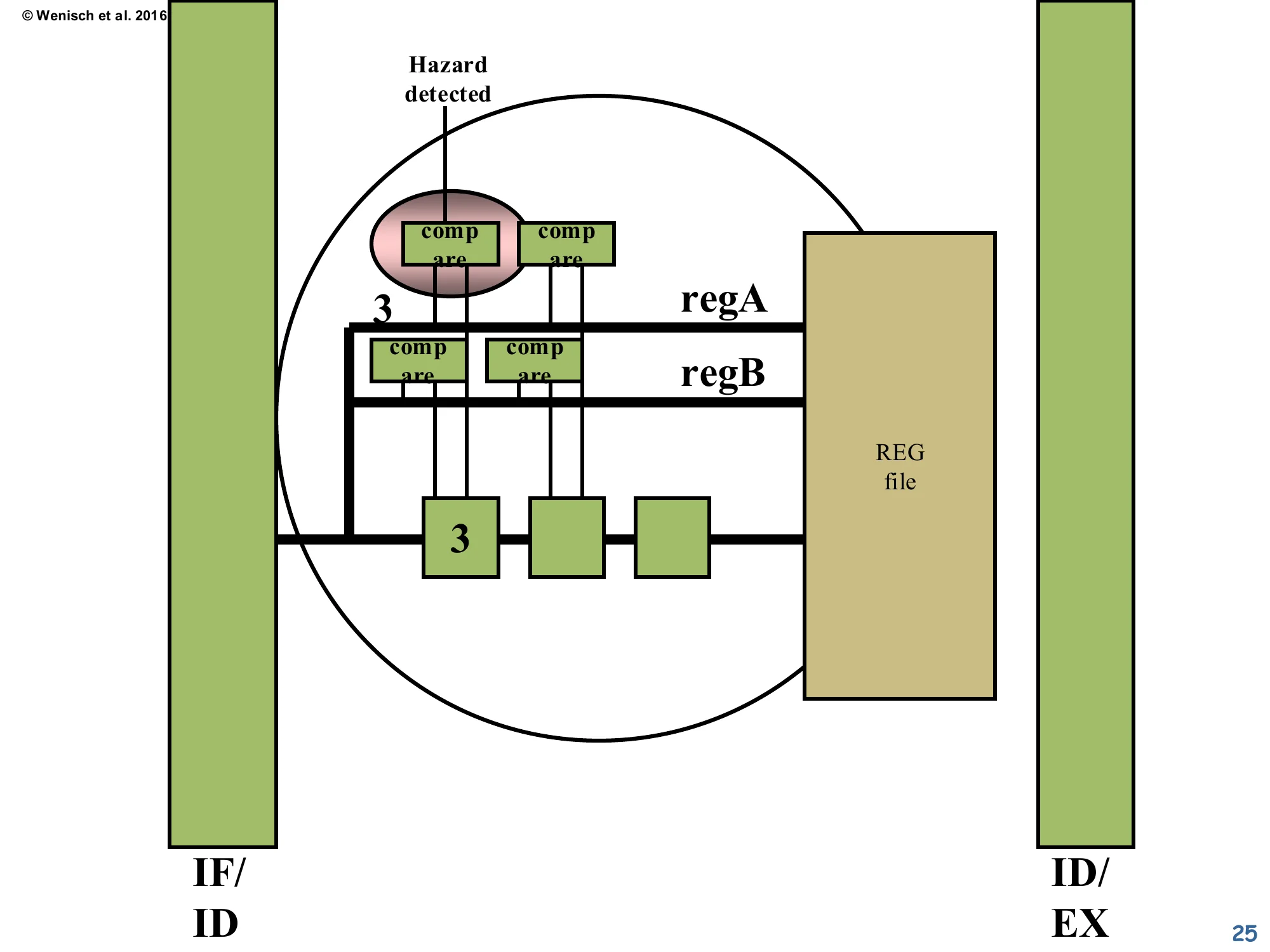
Hazard-detection comparator network (zoomed view, between IF/ID and ID/EX)

Four compare blocks: two compare regA against the three pending dests, two compare regB. The shaded comparator on the left is the one that fires (because regA = 3 matches the dest = 3 sitting in the first ID/EX-stage box). The output of any matching comparator is the Hazard detected signal.

This zoom shows the actual hardware: a 2-deep × 3-stage grid of equality comparators. Each row corresponds to one of the consumer’s two source registers (regA, regB); each column corresponds to one of the three in-flight destinations (in ID/EX, EX/Mem, Mem/WB). Any of the six comparators can independently raise the OR-reduced “Hazard detected” output. The shaded leftmost comparator is the active one for this scenario: regA=3 vs. ID/EX dest=3 → match. Note the diagram uses 3-bit comparators because the ISA has only 8 registers — modern 32- or 64-register ISAs use 5- or 6-bit comparators, still cheap. There’s also a subtle correctness point hidden in the comparators on the right: they check destinations that are further along in the pipeline (EX/Mem, Mem/WB), and those too can be sources of stalls if forwarding isn’t implemented yet.

Single comparator — gate-level view

Show slide text

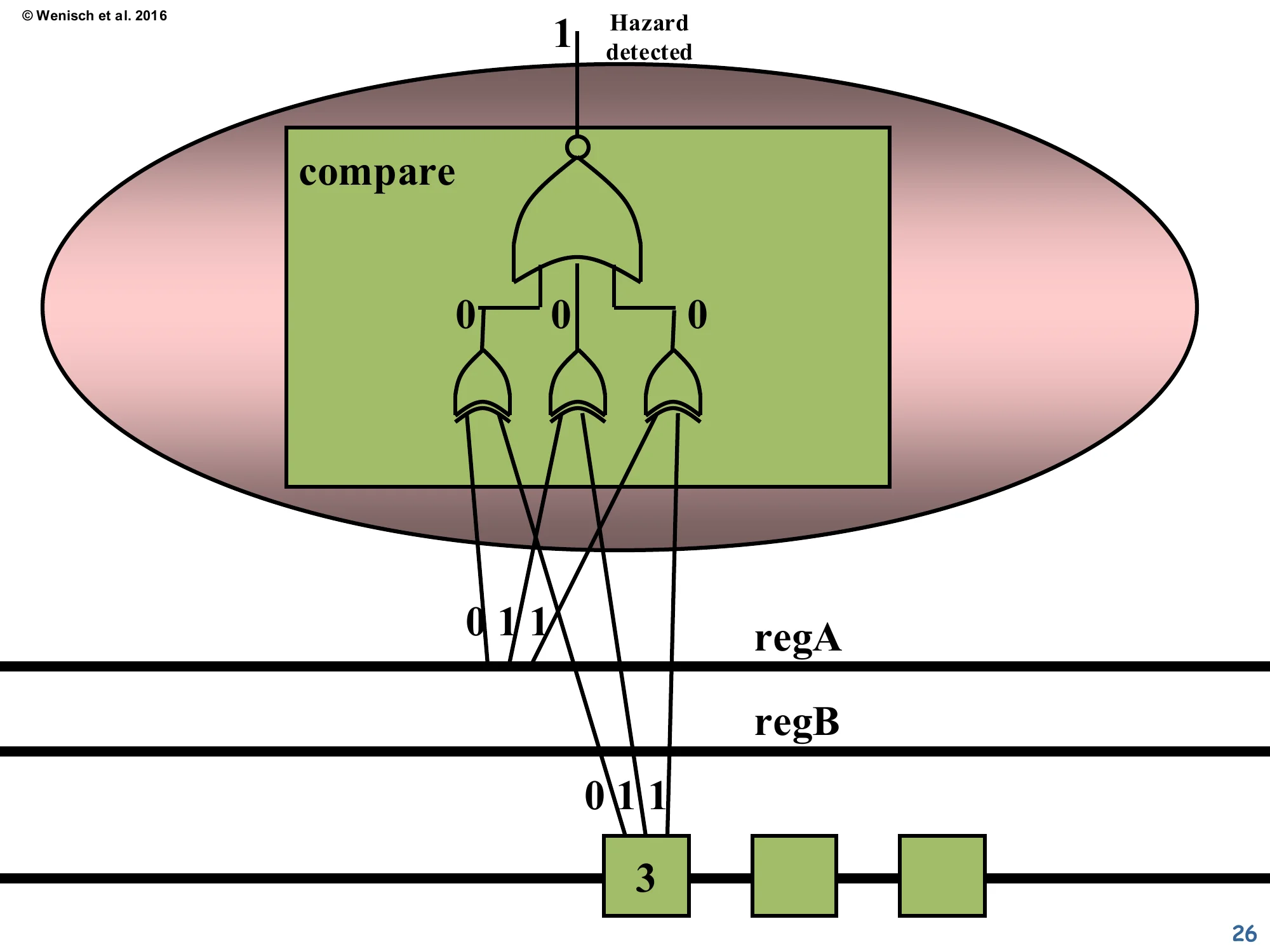
Single comparator — gate-level view

A single compare block is unrolled: three XNOR gates compare each bit of regA against the corresponding bit of dest, then a 3-input AND gate combines them. With regA = 011 (binary 3) and dest = 011, every XNOR outputs 1, the AND outputs 1, and the inverter at the top emits 1 = Hazard detected.

This slide shows the gate-level circuit inside one of the comparators. The XNOR gates (the curved-back gates on the bottom row) output 1 only when the two corresponding bits are equal. AND-ing the three XNOR outputs gives a single “all bits match” signal. The bubble (small open circle) at the very top before the output is just notation: the lecturer draws an inverter so the active-high “hazard detected” output reads cleanly. The total cost is 3 XNOR + 1 AND + 1 NOR per comparator pair (roughly 4–5 standard cells), with 6 comparators total — well under 100 transistors, negligible compared to the rest of the datapath. This is why dynamic interlocks won out over static avoidance: the cost is tiny and it’s invisible to the binary.

First half of cycle 3 — Stall begins

Show slide text

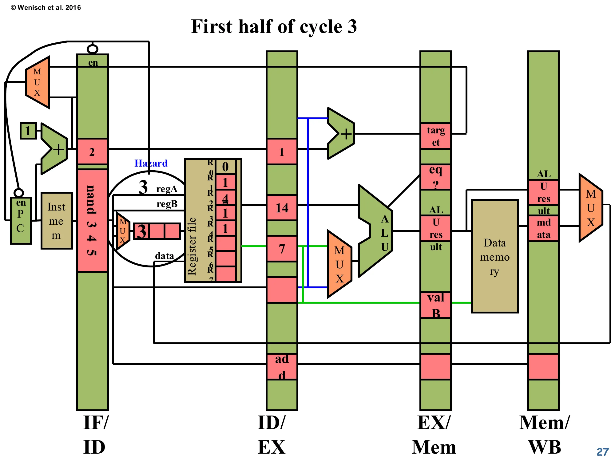
First half of cycle 3 — Stall begins

The Hazard signal is now wired into PC’s enable (via the small enPC block) and IF/ID’s enable (en). Both are de-asserted (note the bubble on the wire), so PC and IF/ID hold their values. The IF/ID latch still shows nand 3 4 5. The ID/EX latch is being prepared to receive a NOP next cycle.

The hazard signal has propagated to the control logic. Two enables are de-asserted: the PC’s enable (so the program counter doesn’t advance — the next instruction stays in instruction memory) and the IF/ID latch’s enable (so nand stays in IF/ID instead of moving forward). The bubble (small circle) drawn on the enable wires indicates active-low semantics — the wire normally carries 1 to allow advancement, and goes to 0 to stall. Meanwhile, the ID/EX latch will be loaded with a no-op encoding at the rising clock edge. The visible add in ID/EX is the producer that’s still flowing forward correctly; what changes is what gets put into ID/EX next cycle.

End of cycle 3 — NOP injected

Show slide text

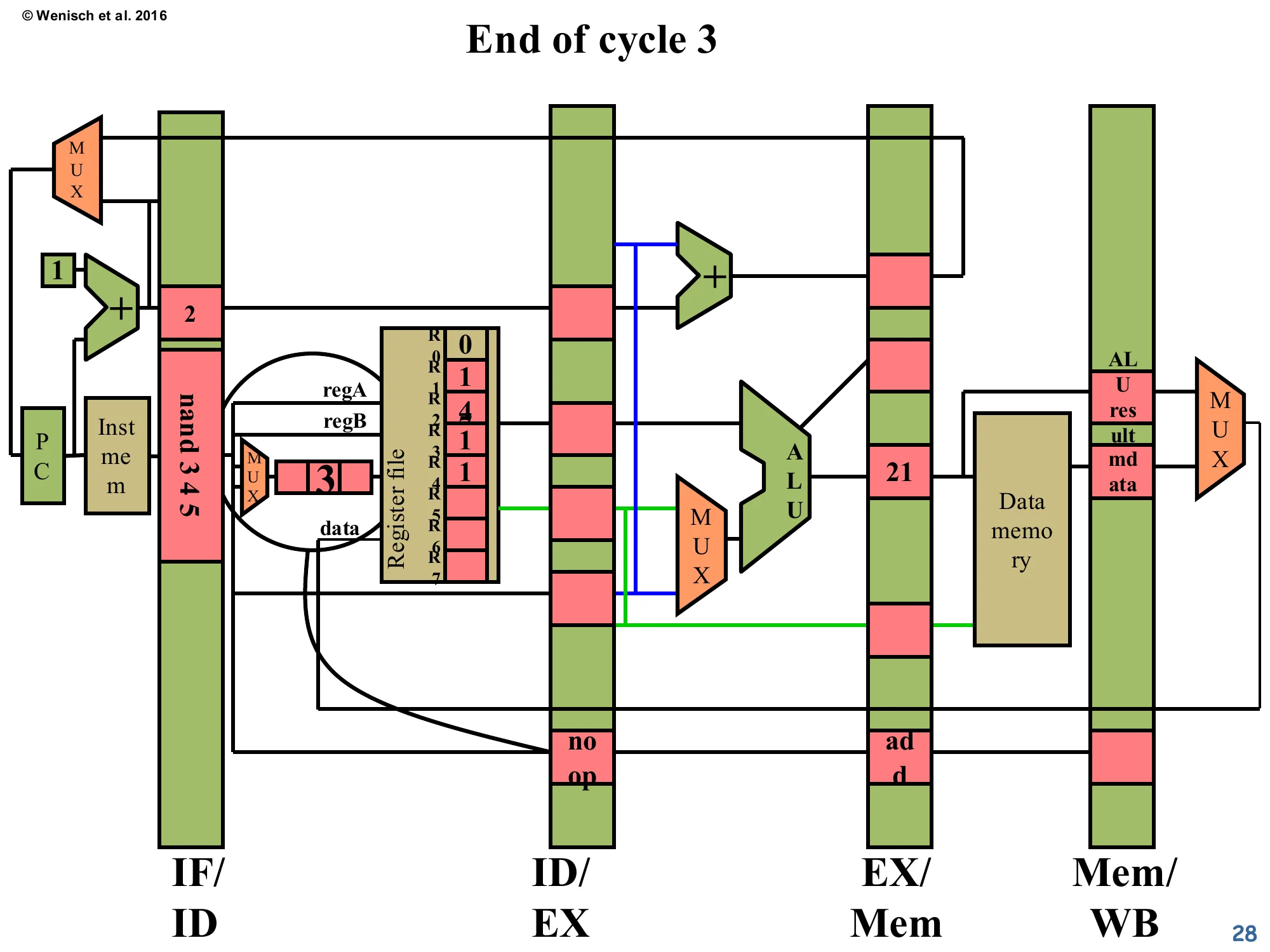
End of cycle 3

ID/EX latch now holds noop (visible at bottom of the latch).
EX/Mem holds the older add with ALU result 21 (the sum 14 + 7 written by EX in this cycle).
IF/ID still holds nand 3 4 5 — it did not advance.
Mem/WB is empty (no instruction has reached WB yet).

The end-of-cycle-3 snapshot shows the bubble in action. The producer add has executed: its ALU produced 21 (= 14 + 7), now sitting in the EX/Mem latch ready for memory access (which is a no-op for an ADD, just passes the value through). ID/EX now holds a noop — that’s the bubble injected when the hazard was detected. IF/ID still holds the consumer nand, frozen by the disabled enable. From the consumer’s perspective, the pipeline has effectively rewound — nand is still waiting in fetch/decode while the rest of the world advances. The cost is one cycle of CPI penalty for this one hazard; multiple back-to-back hazards multiply the cost.

First half of cycle 4 — Hazard still detected

Show slide text

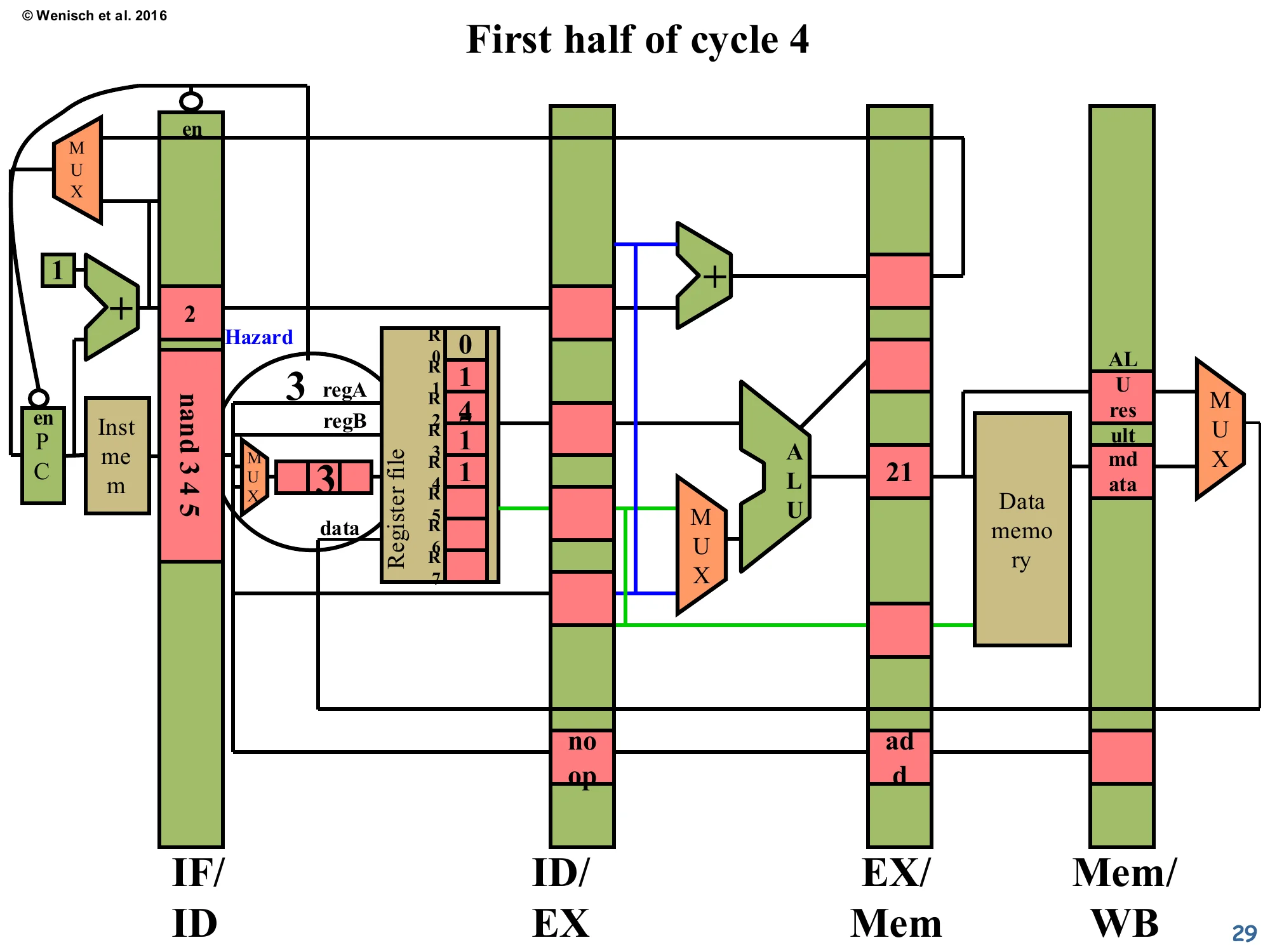
First half of cycle 4 — Hazard still detected

The nand 3 4 5 is still in IF/ID. The detector inspects again: the older add is now in EX/Mem (one stage further along), but dest = 3 is still in flight. The match still fires → Hazard signal asserted again. PC and IF/ID enables are de-asserted again.

One cycle later, the hazard logic re-evaluates — and the answer is still “hazard”. The producer’s destination has migrated from ID/EX to EX/Mem, but it’s still ahead of the consumer in the pipeline, and it still hasn’t reached the WB stage where it would actually update the register file. So the comparator on the EX/Mem-stage dest (the second column of the comparator grid from page 25) lights up. PC and IF/ID stay frozen for another cycle. The pattern is: each cycle that the hazard distance hasn’t yet been bridged, the pipeline spends one more bubble cycle. For this 5-stage pipeline with no forwarding, the consumer must wait until the producer reaches WB — that’s two stall cycles for an immediately-following dependent instruction.

End of cycle 4

Show slide text

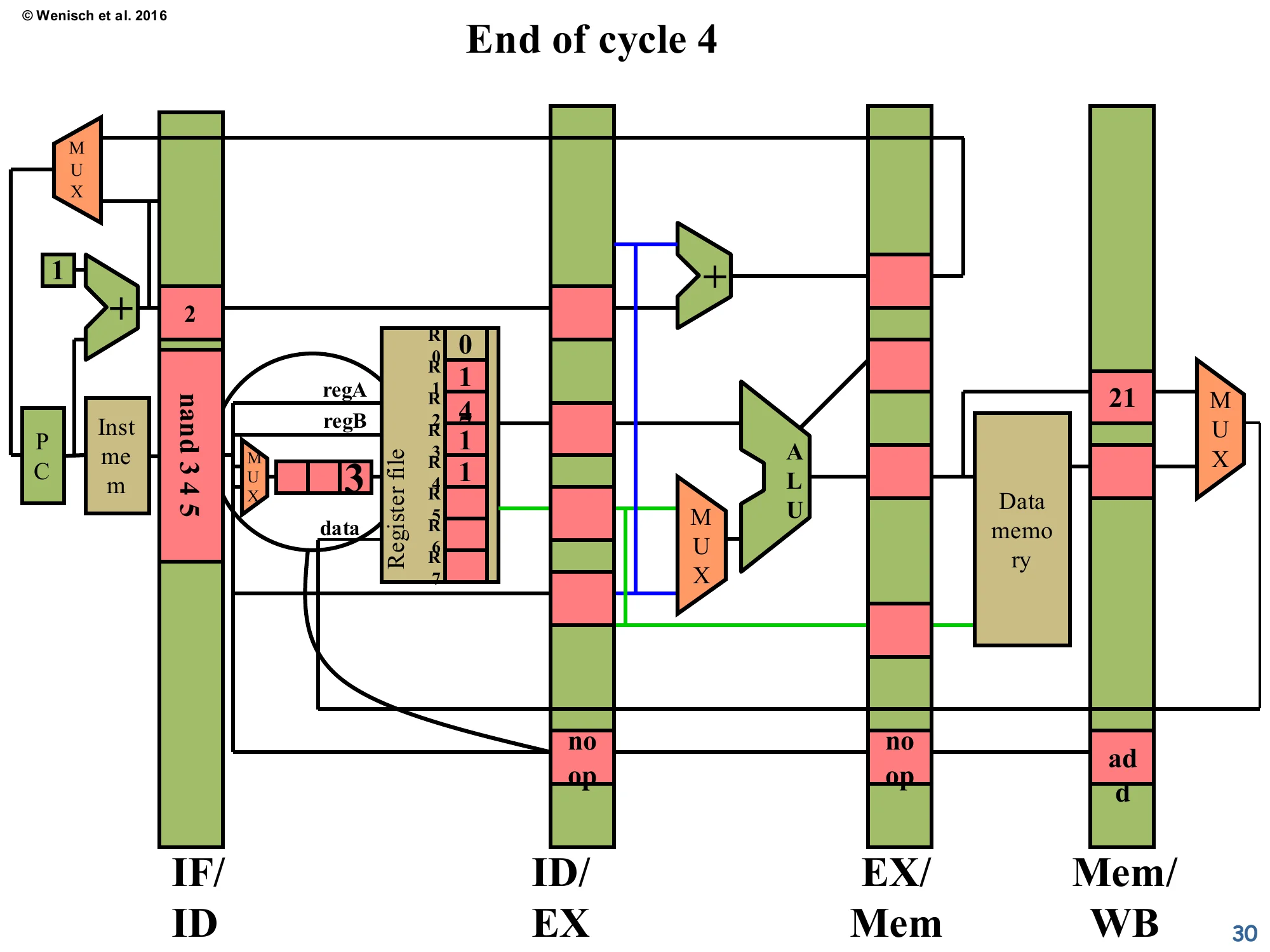
End of cycle 4

ID/EX: another noop inserted.
EX/Mem: now noop (the previous bubble has flowed forward).
Mem/WB: add with ALU result 21.
IF/ID: still nand 3 4 5.

The bubble has propagated one stage (ID/EX → EX/Mem) and a second bubble was just injected into ID/EX. The producer add has reached Mem/WB, holding ALU-result 21 — it’s now one cycle away from writing the register file. The consumer nand is still pinned in IF/ID, having spent two cycles there. Looking at the pipeline as a whole, useful work is happening only in Mem/WB this cycle; ID/EX, EX/Mem are doing nothing. This is the CPI cost of the stall — two wasted issue slots for a single 3-stage-distance RAW hazard, which is exactly what the formula on slide 15 predicts.

First half of cycle 5 — No Hazard

Show slide text

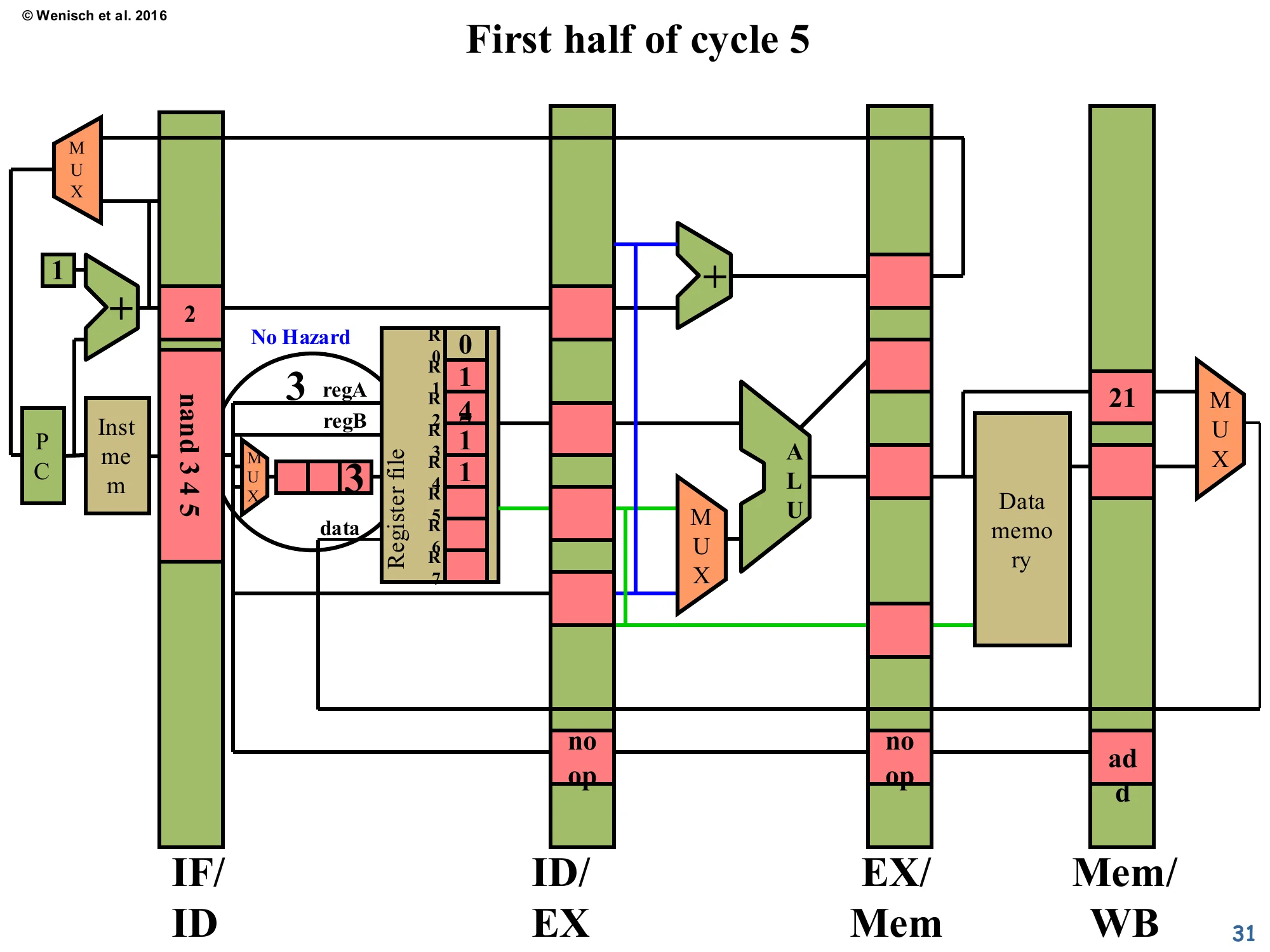
First half of cycle 5 — No Hazard

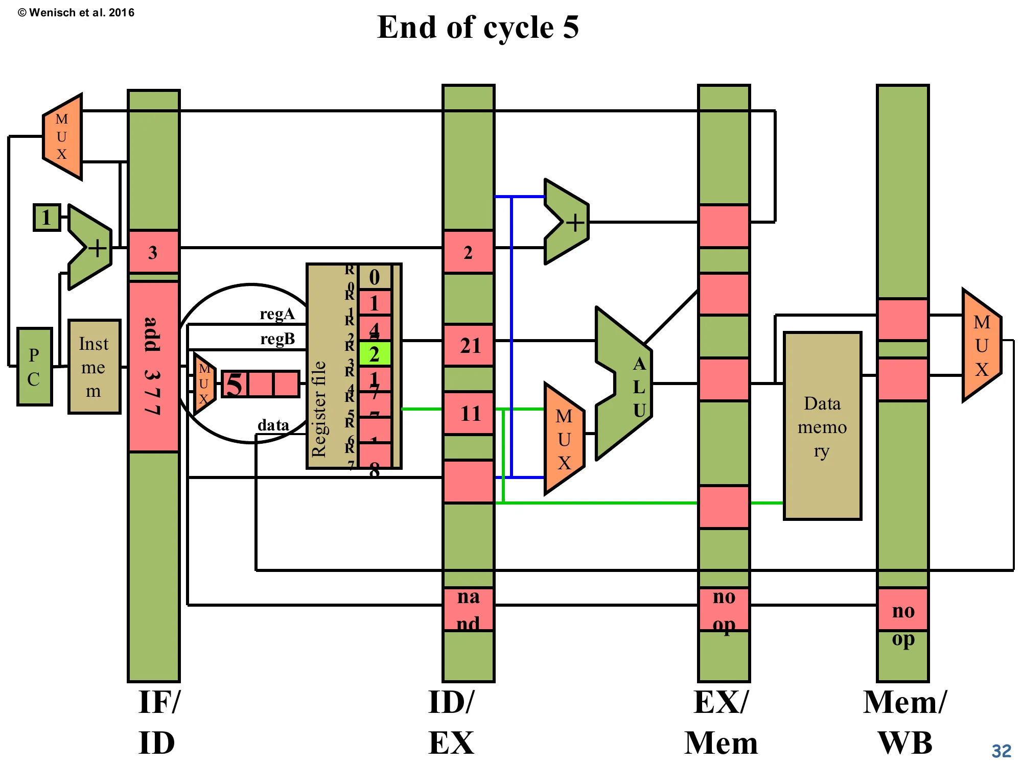
The add is now in Mem/WB and is using the first half of cycle 5 to write 21 into R3 of the register file. The hazard detector fires its comparators again — but because the WB stage simultaneously updates R3, the consumer nand 3 4 5 (still in IF/ID) reads the new value 21 in the second half of cycle 5. Result: No Hazard detected for this cycle, so PC and IF/ID enables are re-asserted.

This slide hinges on a classic implementation trick: write-then-read in the same cycle for the register file. In the first half of cycle 5, the producer’s WB stage writes 21 into R3. In the second half of the same cycle, the consumer’s ID stage reads R3 and gets 21 (not the stale 0). Because the comparator network sees the writeback in progress and accounts for it, the hazard signal goes low and the pipeline resumes. Notice that the register file’s R3 cell is now highlighted with value 2 (the new content; the diagram tracks operand values through the run). Without the half-cycle write/read trick, the consumer would need to wait one more cycle, costing a third bubble. This optimisation is essentially free in modern designs because register-file SRAMs already operate with a write port and a separate read port that can fire in the same cycle.

End of cycle 5

Show slide text

End of cycle 5

IF/ID: a new instruction add 3 7 7 has been fetched (because the pipeline is moving again).
ID/EX: nand 3 4 5 finally advanced into decode → execute, now showing valA=21, valB=11 (R3 freshly read as 21, R4 as 11).
EX/Mem and Mem/WB hold the trailing noop bubbles inserted earlier.

Now the pipeline is back in steady state. The consumer nand 3 4 5 finally has its operands: valA=21 (from R3, freshly written) and valB=11 (from R5… or whatever the example assigns; the structure is what matters). It’s flowing through ID/EX into EX. The two bubbles that filled the gap are still working their way through EX/Mem and Mem/WB — they cause no harm because each bubble carries op=NOP, which the WB stage interprets as “don’t write the register file”. The fetched instruction stream has resumed (add 3 7 7 is now in IF/ID). End of the worked example: a 3-stage RAW hazard cost two cycles of stall in this no-forwarding implementation. The next several slides will redo the same scenario with a forwarding network and show how those two cycles can be reclaimed.

Problems with Detect & Stall

Show slide text

Problems with Detect & Stall

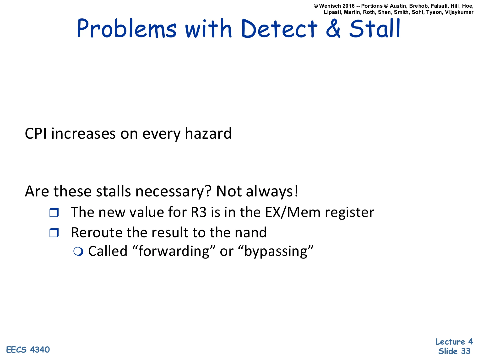
CPI increases on every hazard

Are these stalls necessary? Not always!

The new value for R3 is in the EX/Mem register
Reroute the result to the nand
- Called “forwarding” or “bypassing”

Detect-and-stall is correct but pessimistic. The slide highlights the key insight: even though the producer’s value isn’t yet in the architectural register file, the value already exists somewhere in the pipeline — in the EX/Mem latch as the ALU result, or in Mem/WB as either the ALU result or the loaded data. So instead of stalling the consumer until WB completes, we can route (forward / bypass) the value directly from those latches to the consumer’s ALU input MUX. This reduces the CPI penalty for a typical add→use hazard from 2 cycles down to 0 — the consumer no longer has to stall at all. The remaining cost is the new MUXes in front of the ALU (selecting between register-file output, EX/Mem-forwarded value, Mem/WB-forwarded value) and the wires to carry the bypassed values back to the front. The next several slides walk through the worked example again with this forwarding network in place.

Handling Data Hazards: Detect & Forward

Show slide text

Handling Data Hazards: Detect & Forward

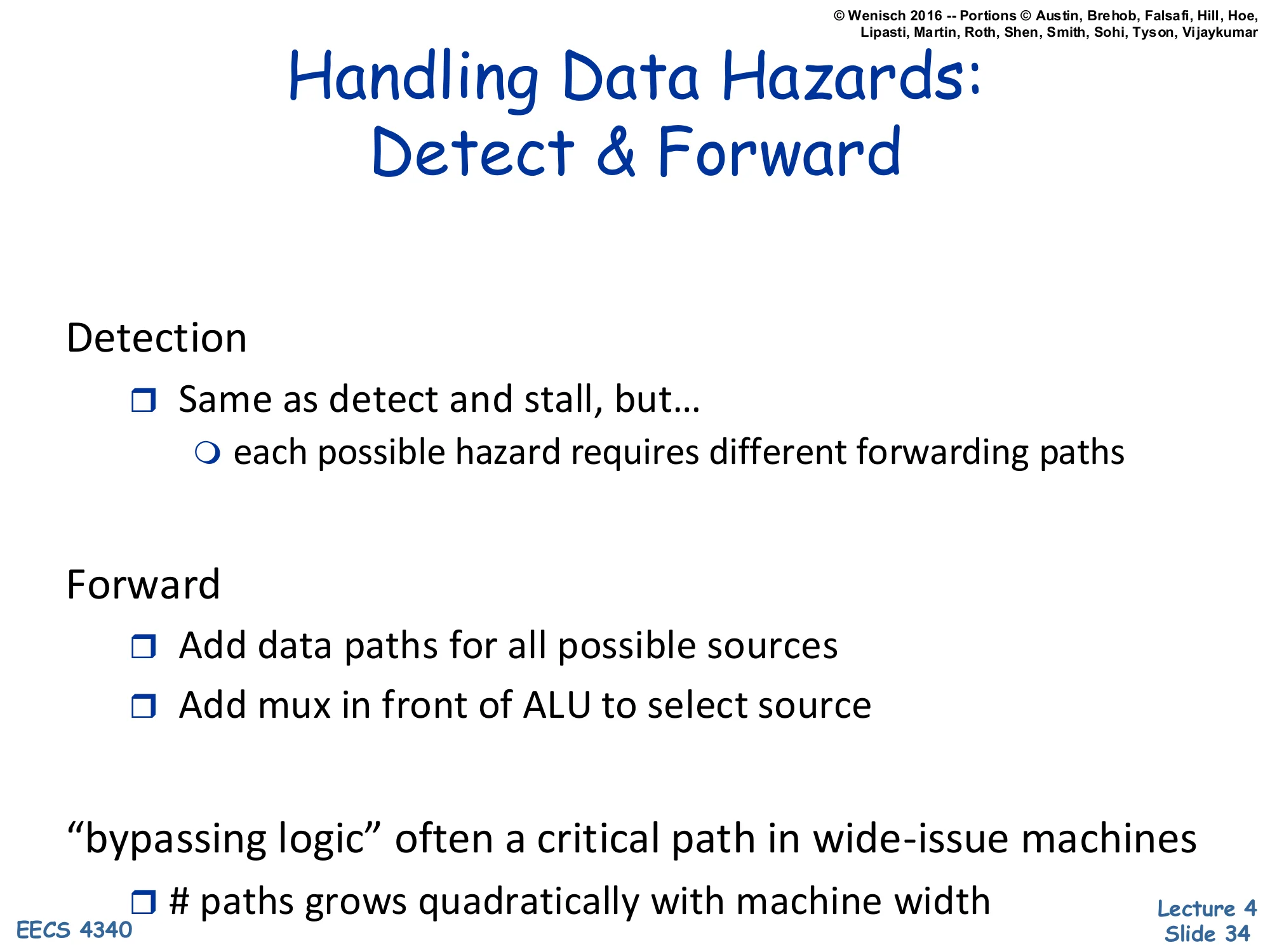
Detection

Same as detect and stall, but…
- each possible hazard requires different forwarding paths

Forward

Add data paths for all possible sources
Add mux in front of ALU to select source

“bypassing logic” often a critical path in wide-issue machines

paths grows quadratically with machine width

Detect-and-forward generalises detect-and-stall: instead of converting a hazard into a bubble, you convert it into a different routing decision. Detection is essentially the same comparator network — but now each comparator’s output, rather than enabling a stall, drives a select signal on the new MUX in front of the ALU. Forwarding paths must exist for every place a producer might be: at minimum EX/Mem→ALU-input and Mem/WB→ALU-input. Each such path is a wide bus running across most of the datapath. The slide flags the cost: in a wide-issue OoO machine with N parallel ALUs, every ALU input MUX needs $\mathcal{O}(N)$ inputs (one per other ALU’s output), so the total wire count grows as $\mathcal{O}(N^2)$ . This bypass network is a notorious critical path in modern processors and is one of the reasons wide-issue cores have stalled around 4–6 wide rather than continuing to scale up.

First half of cycle 3 (with forwarding)

Show slide text

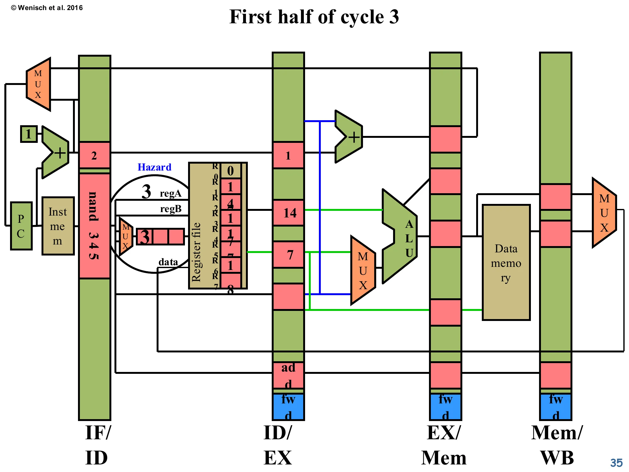
First half of cycle 3 (Detect & Forward)

New blue fwd boxes are visible at the bottom of the EX/Mem and Mem/WB latches — these carry the forward-control signals. The Hazard circle still fires on the same comparator match (nand’s regA = 3 vs. add’s dest = 3 in ID/EX) but the response will be different: instead of stalling, the pipeline will route the add’s ALU result around to the nand’s ALU input.

We replay the same producer/consumer scenario, but with the forwarding network added. The new blue fwd flip-flops at the bottom of EX/Mem, Mem/WB (and the corresponding fwd field in ID/EX, just appearing in the next slide) hold control signals that tell the new ALU-input MUX which forwarding source to pick. The detection logic itself is unchanged — same comparator network — but its output is now repurposed: instead of asserting a stall on PC/IF/ID, it asserts the appropriate fwd select line, which is propagated along with the consumer down the pipeline. The hazard is detected at end-of-cycle-2 / first-half-cycle-3, exactly as before, but no stall is generated.

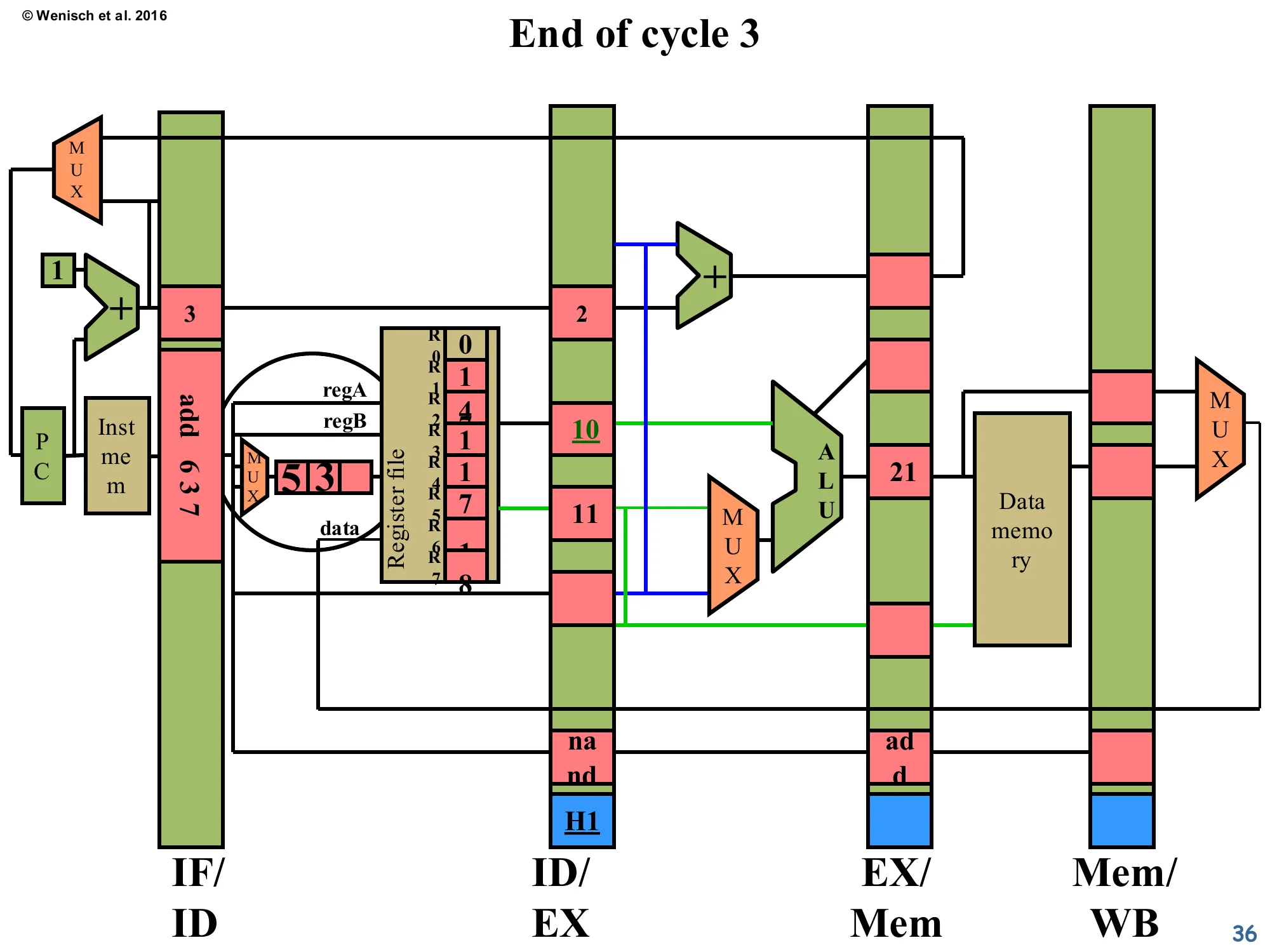
End of cycle 3 (forwarding propagated)

Show slide text

End of cycle 3

IF/ID: new instruction add 6 3 7 has just been fetched.
ID/EX: nand 3 4 5 has advanced into decode → entering EX next cycle. Its valA slot reads 10 (from regA=3, but R3 isn’t written yet — value is stale!). Below the latch, the new H1 label marks the forwarding-control signal that will tell EX’s ALU MUX to ignore valA and instead grab the forwarded value from EX/Mem.
EX/Mem: add with ALU result 21.

The pipeline has not stalled. The consumer nand advanced into ID/EX even though R3 hasn’t been written yet, and its valA slot now contains the stale value 10 read straight from the register file. This would normally be wrong — except that the H1 forwarding-control bit (newly visible at the bottom of the ID/EX latch) is set, and it tells the ALU input MUX next cycle to discard valA and instead use the value coming out of EX/Mem (which is the producer’s ALU result, 21). The producer add has migrated to EX/Mem with its result intact. A new instruction add 6 3 7 has entered fetch — note this introduces a second hazard against the consumer (the new add reads R3, which nand just wrote!). The next slide handles that second hazard.

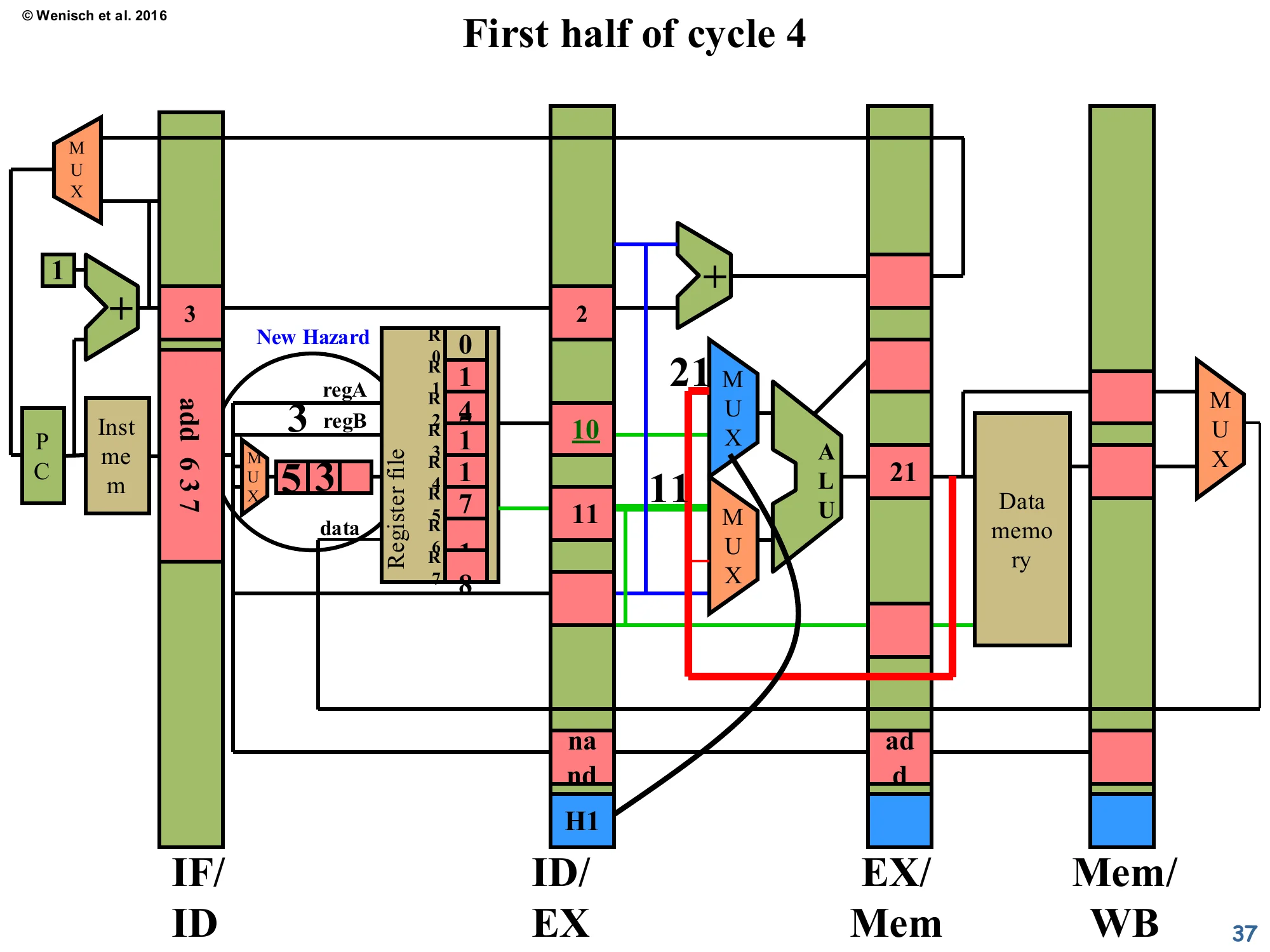
First half of cycle 4 — Forward + new hazard

Show slide text

First half of cycle 4

The blue MUX in front of the ALU is now drawn explicitly. Two red-highlighted forwarding wires fan in from EX/Mem (carrying ALU result 21) into both ALU input MUXes. Black control wires from the H1 field in ID/EX select “forward from EX/Mem” instead of valA.
Decode also detects a New Hazard: the freshly-fetched add 6 3 7 reads R3, which nand (now in ID/EX) is about to write. So a second forwarding event — H2 — will be needed for the next cycle.

This is the full picture of forwarding. The red wires sweeping from EX/Mem back to the ALU inputs are the forwarding bus. The blue MUX in front of the ALU now picks among (i) regular valA from ID/EX, (ii) forwarded value from EX/Mem, (iii) forwarded value from Mem/WB. The H1 bit selects option (ii) for valA in this cycle. Simultaneously, decode discovers a new hazard for the next-younger instruction add 6 3 7 against nand’s about-to-be-computed R3 — so a second forwarding setup (H2) is queued up. The lecturer’s point: in a real pipeline you can have multiple concurrent hazards on different stages simultaneously, and the forwarding network must handle all of them in parallel. This is also why the bypass network area scales as $\mathcal{O}(N^2)$ in machine width — any producer-stage might be the source for any consumer-stage.

End of cycle 4 (forwarding active)

Show slide text

End of cycle 4

ID/EX: now contains the third instruction lw 3 6 10. Forwarding-control field shows H2 set.
EX/Mem: the nand has executed; ALU result is −2 (= 21 NAND 11, written through the forwarded path). Below: H1 propagates forward.
Mem/WB: add with result 21, now ready for writeback.

The forwarding worked — nand produced its output −2 in cycle 4, with no stall cycles, by consuming the producer’s result directly from EX/Mem. Compare to the no-forwarding trace (page 28–32) where nand was stalled for two cycles. The forwarding-control bits move forward along with each instruction so that subsequent stages can re-check whether they too should source from a forwarded value. The consumer’s now-complete ALU result −2 is sitting in EX/Mem, where it can serve as a forwarding source for the next dependent instruction (the H2 marker on ID/EX is preparing for exactly that).

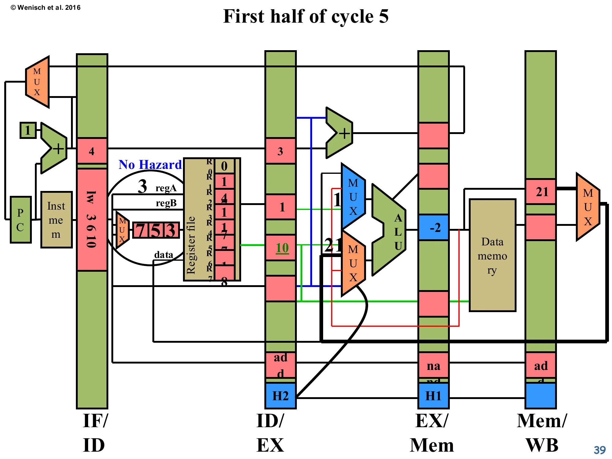
First half of cycle 5 (cascaded forwarding)

Show slide text

First half of cycle 5

IF/ID: new instruction (sw) being fetched. Decode reports No Hazard for it.
ID/EX: lw 3 6 10 — its valA slot needs R3, which is now −2 in EX/Mem. The H2 bit selects the forwarded path (red wire) so the ALU MUX picks −2 instead of the stale register-file value.
EX/Mem: nand with result −2.
Mem/WB: add with result 21.

Cascaded forwarding: lw is the third instruction in the dependency chain (it reads R3 which nand just wrote). H2 routes nand’s −2 from EX/Mem to lw’s ALU input — for free, no stall. Notice the diagram now shows two simultaneous forwarding events drawn as red overlays: one feeding lw’s ALU input from EX/Mem, and one (the older H1) carrying add’s result through Mem/WB. This illustrates why the bypass network scales quadratically: every consumer in the pipeline might be sourcing from every producer further along, and every such pair needs its own wire and MUX input. For this 5-stage in-order pipeline the cost is still manageable; for a 4-wide OoO machine, the bypass wires dominate the back-end floorplan.

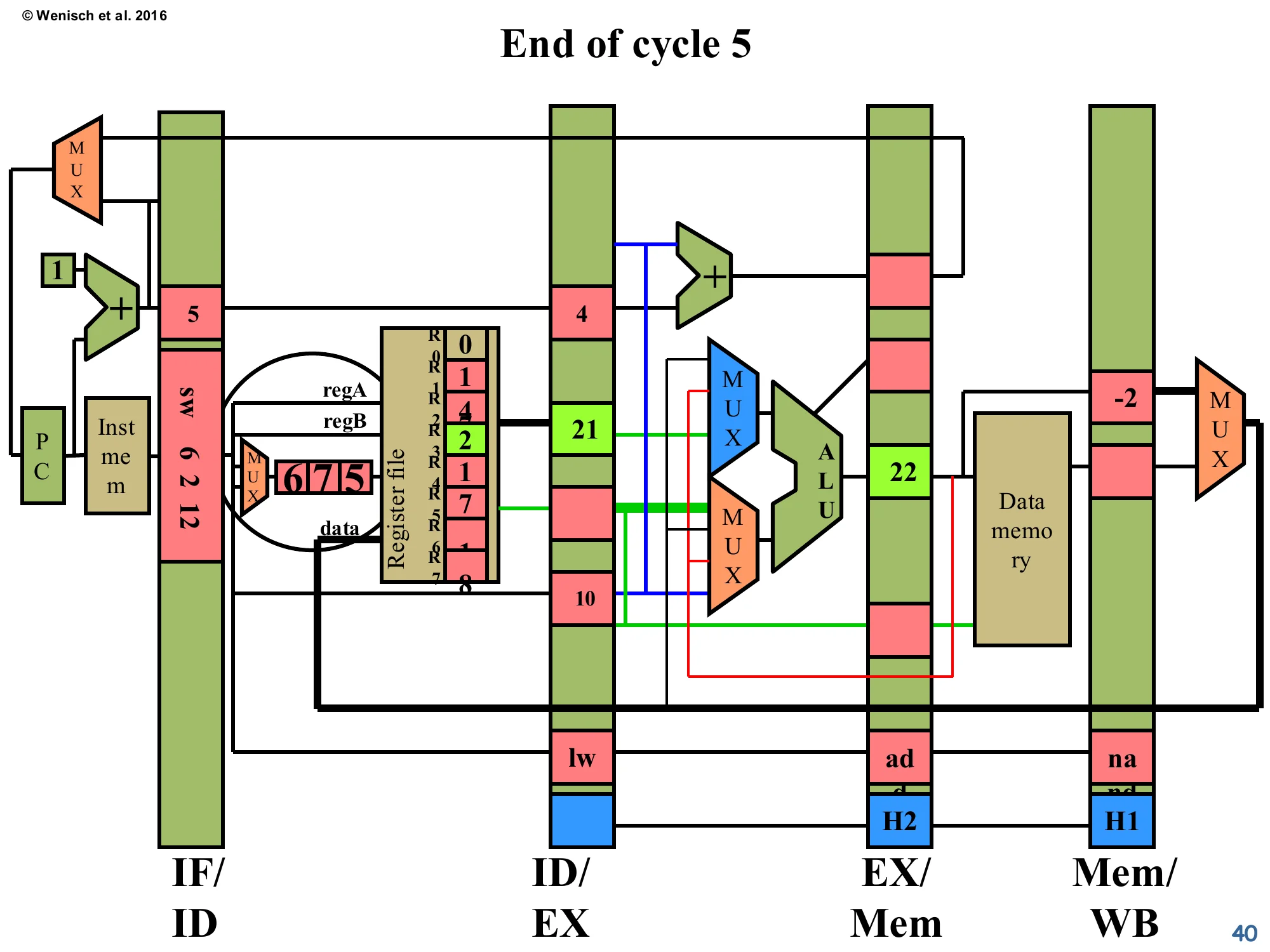
End of cycle 5

Show slide text

End of cycle 5

IF/ID: sw 6 2 12 fetched.
ID/EX: third instruction now sitting in decode→execute, reading R3 = 21 from the freshly-written register file (the original add retired in WB this cycle).
EX/Mem: lw with ALU-computed effective address 22.
Mem/WB: nand with result −2.
The register file shows R3 freshly written with the value 2 in this snapshot.

Steady-state pipeline operation continues. Five instructions are in flight, each in a different stage. The original add has just retired; nand’s −2 is in WB and will retire next cycle. lw’s ALU has computed an effective address (R3 + 10 = 21 + 10 = 31 in the lecturer’s running example — the 22 in the diagram comes from the example’s specific values). With forwarding fully engaged, CPI is back to the ideal 1.0 for this dependency chain — no stalls were ever issued. The next slide will reveal a special case where forwarding alone is not sufficient: a load-use hazard.

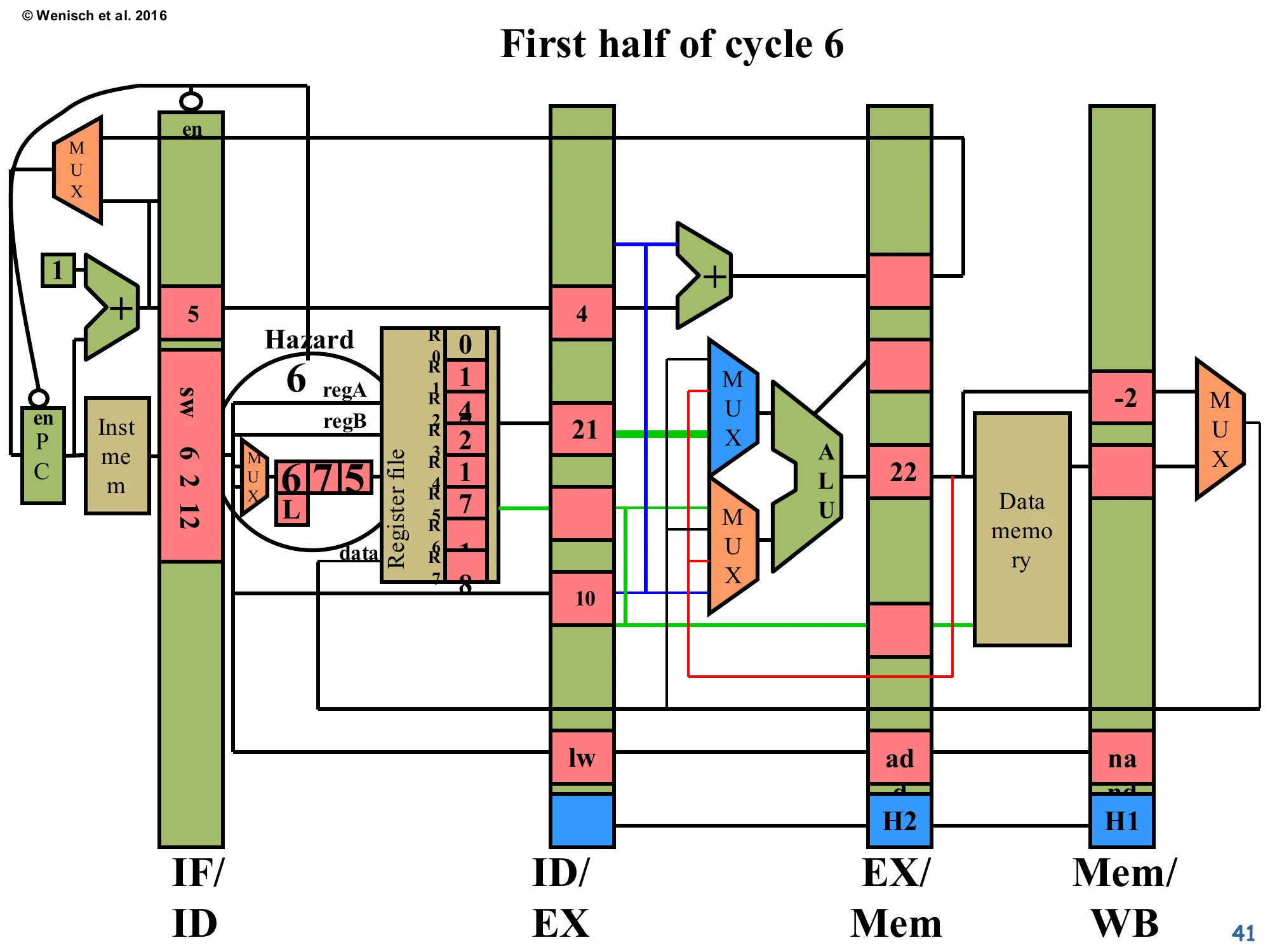
First half of cycle 6 — Load-use hazard

Show slide text

First half of cycle 6

IF/ID: sw 6 2 12 — its regA=6 matches lw 3 6 10’s dest=3? No, but it does need R6. The lecturer’s diagram now flags Hazard because sw’s regA = 6 matches… wait, the visible label is sw 6 2 12 with regA=6. The crucial new feature: a small L flag on the H field next to the ID/EX latch — marking that this hazard cannot be resolved by EX/Mem-stage forwarding because the producer is a load, whose data is only available at the end of MEM, one cycle later than for an ALU result.
Therefore PC and IF/ID are again stalled (en signals de-asserted).

This slide introduces the famous load-use hazard. The producer lw (load word) doesn’t compute its result in EX — EX only computes the effective address. The actual loaded data isn’t available until the end of MEM. So if the very next instruction depends on the loaded value, there is no source latch with the data ready in time for the consumer’s ALU. Forwarding can’t manufacture the data out of thin air; the consumer must stall for exactly one cycle. The L marker (“Load” hazard) on the forwarding-control bit signals exactly this case to the front-end, telling it to freeze IF/ID and PC for one cycle. After that one bubble, the loaded value is in Mem/WB and can be forwarded normally to the now-advanced consumer. This is why early MIPS designs exposed a load delay slot in the ISA — they punted the bubble-injection responsibility back to the compiler. Modern designs always have this stall in hardware.

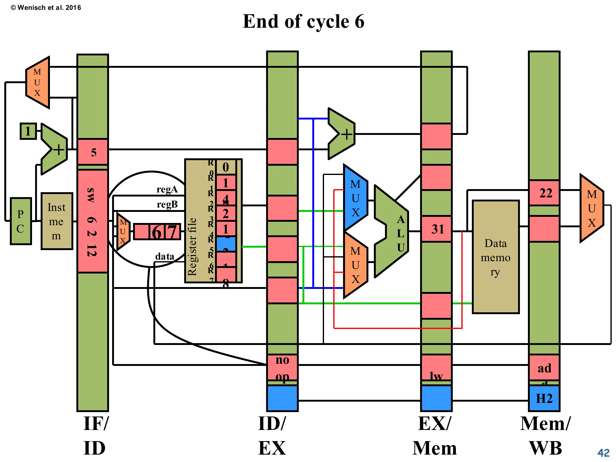
End of cycle 6 (load bubble injected)

Show slide text

End of cycle 6

IF/ID: sw 6 2 12 still pinned in fetch (frozen by the load-use stall last cycle).
ID/EX: noop injected (visible at bottom). Forwarding fields show H2 still propagating.
EX/Mem: lw with computed address 31, about to access data memory.
Mem/WB: add with 21.

The load-use stall has produced exactly one bubble — the noop now in ID/EX. The consumer sw is still pinned in fetch waiting for the load’s data. The producer lw is in EX/Mem with its computed address (R3 + 10 = 21 + 10 = 31); next cycle it will issue the memory read and place the loaded data in Mem/WB. Once that happens, forwarding from Mem/WB can supply the consumer in EX. The total cost: one cycle of stall per load-use hazard. Compare to: a non-load RAW hazard (forwarded from EX/Mem) costs zero cycles, and a load-use hazard costs one cycle. This is why compiler scheduling still matters for performance even on modern out-of-order CPUs — getting the dependent instruction one slot later in the schedule converts a 1-cycle stall into a 0-cycle stall.

First half of cycle 7

Show slide text

First half of cycle 7

The hazard re-evaluates: the lw is now one stage further (Mem/WB), but the loaded data is still being fetched from data memory. The Hazard label still fires because the consumer’s source is now compared against Mem/WB’s dest. However the H2 control already promotes forwarding from Mem/WB.
IF/ID still holds sw 6 2 12.
ID/EX: noop.
EX/Mem: noop propagated forward.

The pipeline is still managing the load-use scenario. Mid-way through cycle 7, the loaded data has just become available at the output of data memory and is being captured into the Mem/WB latch. The forwarding-control logic will now route that loaded data, in the next half-cycle, into the consumer sw’s ALU input MUX as soon as sw advances into ID/EX. Detection logic confirms this is now solvable via Mem/WB→ALU forwarding rather than via stalling — so the IF/ID and PC enables will be re-asserted at the cycle boundary.

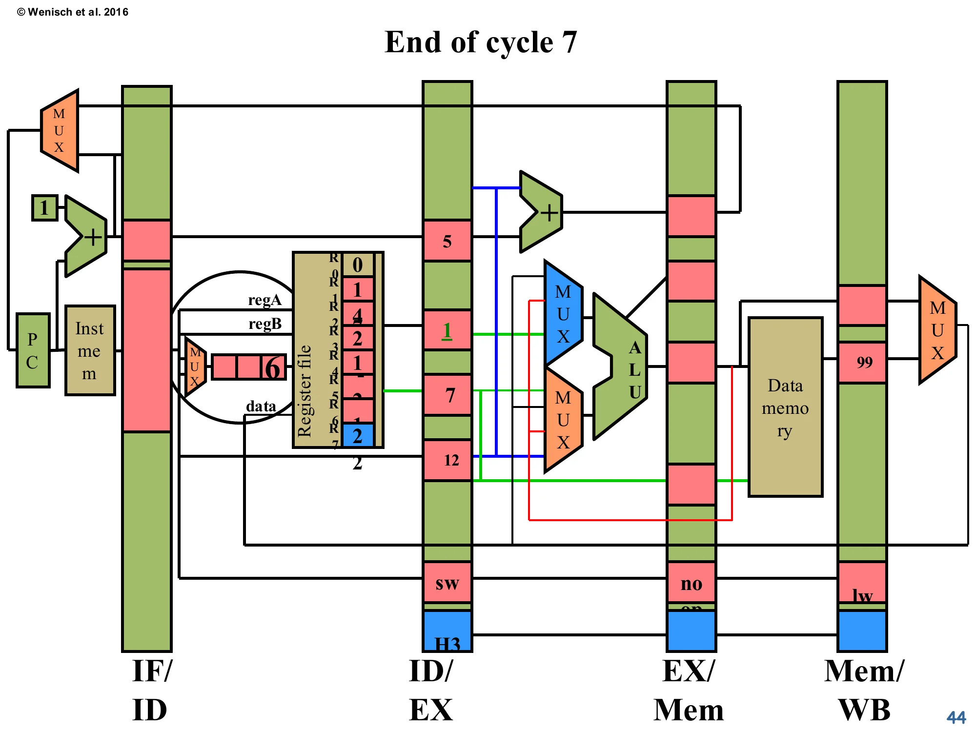
End of cycle 7

Show slide text

End of cycle 7

IF/ID: now empty (or holds the next sequential instruction; the diagram is grayed).
ID/EX: sw 6 2 12 finally advanced. Its valA = 1 (R6’s old value, the −2 is now in R5 of the register file from nand’s WB), and forwarding control H3 marks that it will source R7’s value from the Mem/WB latch holding the loaded data 99.
EX/Mem: noop.
Mem/WB: lw with 99 loaded from data memory (visible in the latch’s mdata field).

Now the consumer sw has finally entered ID/EX and is using forwarded data from Mem/WB. The H3 forwarding-control bit selects “forward mdata from Mem/WB” for the appropriate operand. The loaded value 99 is in the Mem/WB latch. Notice how the trailing noop (the bubble injected during the load-use stall) is sitting in EX/Mem doing no harm. Total stall cost for the load-use hazard: 1 cycle. The pipeline is back at IPC=1 from cycle 8 onward.

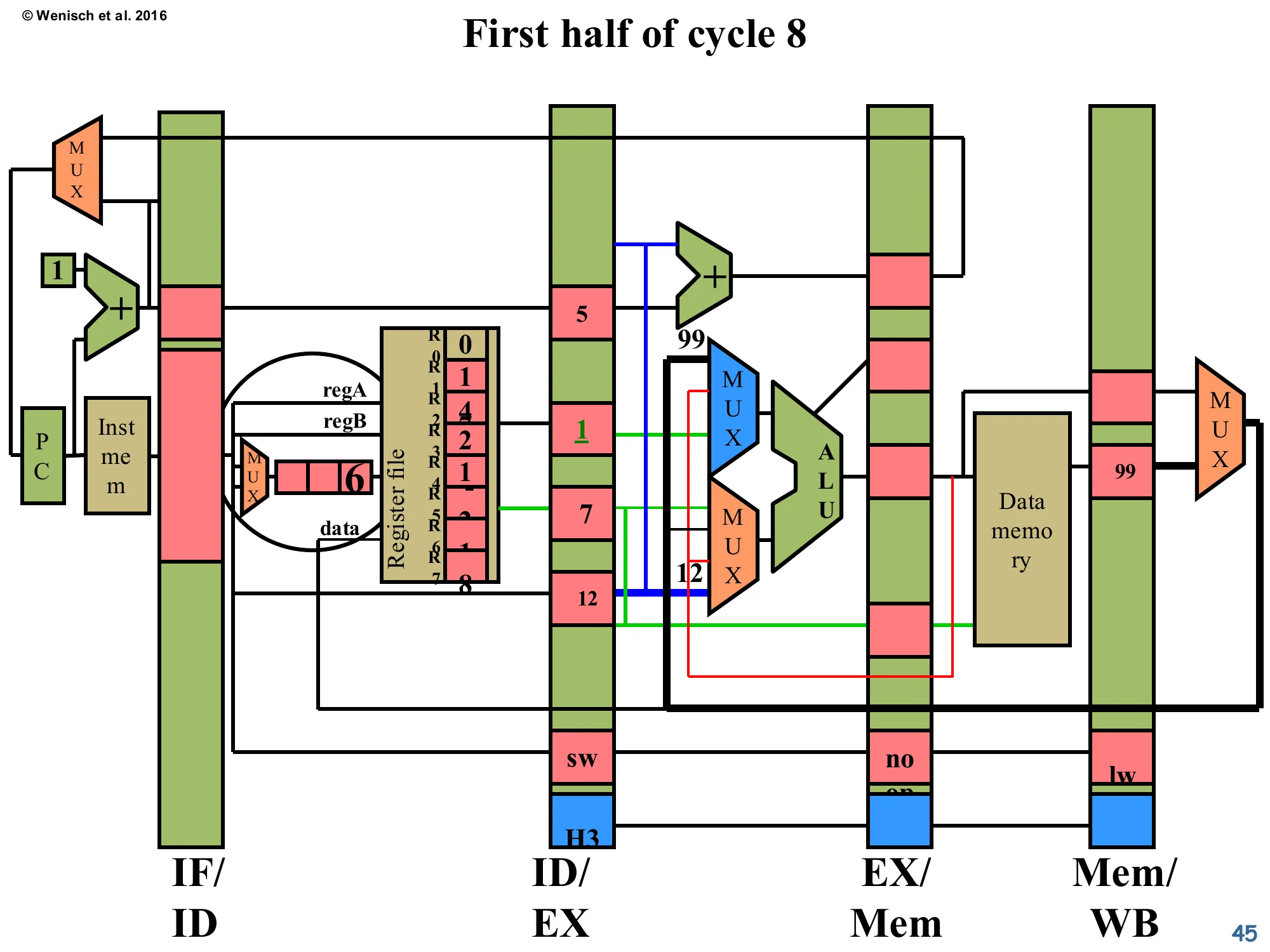
First half of cycle 8 (Mem/WB → ALU forwarding)

Show slide text

First half of cycle 8

The sw’s regA forward path (red wire) now sources the value 99 from Mem/WB and routes it through the ALU input MUX. The ALU effective-address computation will use this forwarded value. EX/Mem latch is empty (the trailing noop has been overwritten).

The forwarding network completes its job for the load-use case. The sw’s ALU input takes the loaded value 99 directly from Mem/WB, computes its effective address, and proceeds to memory. From this cycle onward, the pipeline is at full throughput again. Step back and observe the overall pattern: of the four-instruction sequence (add → nand → lw → sw), the only stall was the one caused by the load→use combination of lw and sw. Every other RAW hazard was forwarded for free. This is why forwarding is the default in every textbook 5-stage pipeline and a key part of any modern processor.

End of cycle 8

Show slide text

End of cycle 8

ID/EX: empty (next instruction fetched, but not shown).
EX/Mem: sw with computed store address 11 and value to store.
Mem/WB: noop (the bubble from the load-use hazard finally retiring).
Register file shows updated state: R5 = 9 (nand’s −2 extended? actually the diagram tracks specific values; the structure is what matters).

Final snapshot of the worked example. The store has computed its effective address using the forwarded loaded value, and is now sitting in EX/Mem ready to actually write to memory in cycle 9 (its MEM stage). The trailing bubble from the earlier load-use stall is harmlessly retiring through Mem/WB. Total cycles for four instructions: 4 (warmup) + 4 (steady-state) + 1 (load-use stall) = 9. Compared to the no-forwarding implementation that would have spent 2 cycles stalling on the add→nand pair plus more on the others, this is a substantial improvement. The lecture has now covered detect-and-stall and detect-and-forward in full. The next slide pivots from data hazards to a different topic: how the original MIPS R2000 turned the load-use hazard into an architectural feature.

Load Delay Slot (MIPS R2000)

Show slide text

Load Delay Slot (MIPS R2000)

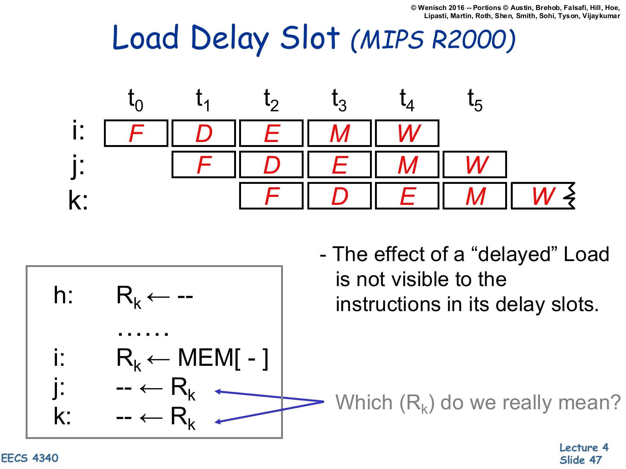
Pipeline trace:

Insn	t0	t1	t2	t3	t4	t5
i:	F	D	E	M	W
j:		F	D	E	M	W
k:			F	D	E	M

Code:

h:  Rk ← --
...
i:  Rk ← MEM[ - ]
j:  -- ← Rk
k:  -- ← Rk

The effect of a “delayed” Load is not visible to the instructions in its delay slots.
Which (Rk) do we really mean? — for j: the old value (from instruction h); for k (and later): the new loaded value.

This slide describes the load delay slot ISA convention used by the original MIPS R2000. The hardware did not implement a load-use stall — instead the architecture declared that the instruction immediately following a load (the “delay slot” instruction) sees the old value of the loaded register, not the newly-loaded one. The compiler is then responsible for either filling the delay slot with an instruction that doesn’t depend on the load, or inserting an explicit NOP. From the timing diagram: instruction i issues a load that produces R_k at the end of cycle 4 (M); instruction j reads R_k in its decode stage at cycle 2, where the old value (from instruction h) is still in the register file; instruction k reads R_k in cycle 3, by which point the new value is committed. This was a fragile design — it broke binary compatibility when later MIPS implementations changed pipeline depth — and was eventually deprecated. The same idea recurs for branches as the branch delay slot (slide 56).

Control Hazards

Show slide text

Control Hazards

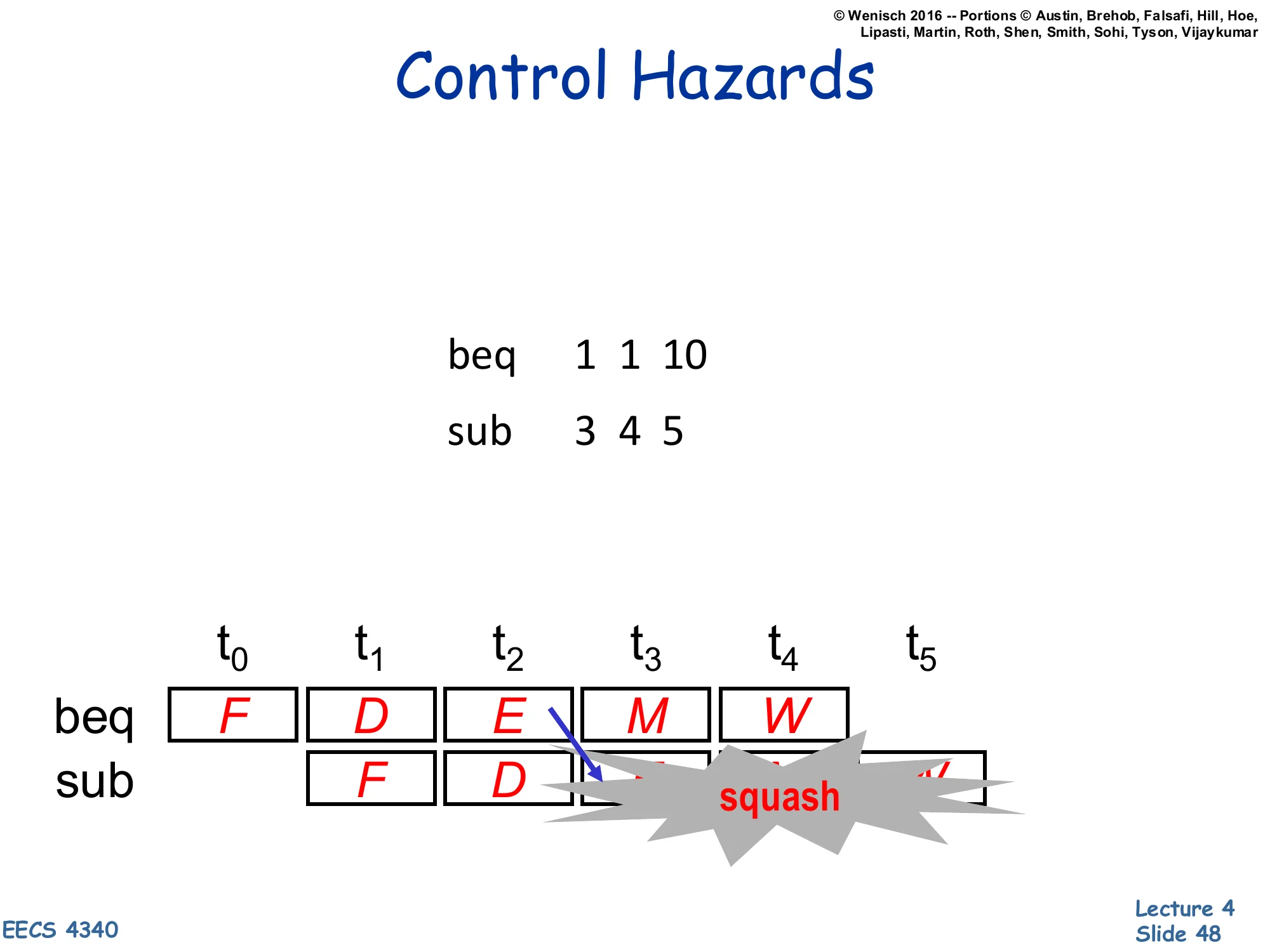
beq  1 1 10
sub  3 4 5

Pipeline trace:

Insn	t0	t1	t2	t3	t4	t5
beq	F	D	E	M	W
sub		F	D	squash	squash	squash

The sub is fetched and decoded before the branch direction is resolved in EX (cycle 3). When the branch is resolved as taken, the speculatively-fetched sub must be squashed.

This slide pivots from data hazards to control hazards. The branch beq 1 1 10 is unconditionally taken (1==1), so execution should jump 10 instructions ahead — but the front end has already fetched the sequentially-following sub 3 4 5 and started decoding it. The branch direction is computed in the EX stage (cycle 3 for beq), and only at that point does the pipeline know which instruction should actually be in fetch. Until then, the pipeline is speculatively executing sub based on the assumption that the branch is not taken. When the assumption turns out to be wrong, every speculatively-executed instruction must be squashed — overwritten with NOPs in the pipeline latches before they can update architectural state. The grey “squash” boxes show this in the trace. Each squashed instruction is one cycle of CPI penalty. Mitigations covered next: prediction, predication, and speculate-and-squash. The taxonomy from page 13 listed control dependence as a distinct category for exactly this reason.

Handling Control Hazards

Show slide text

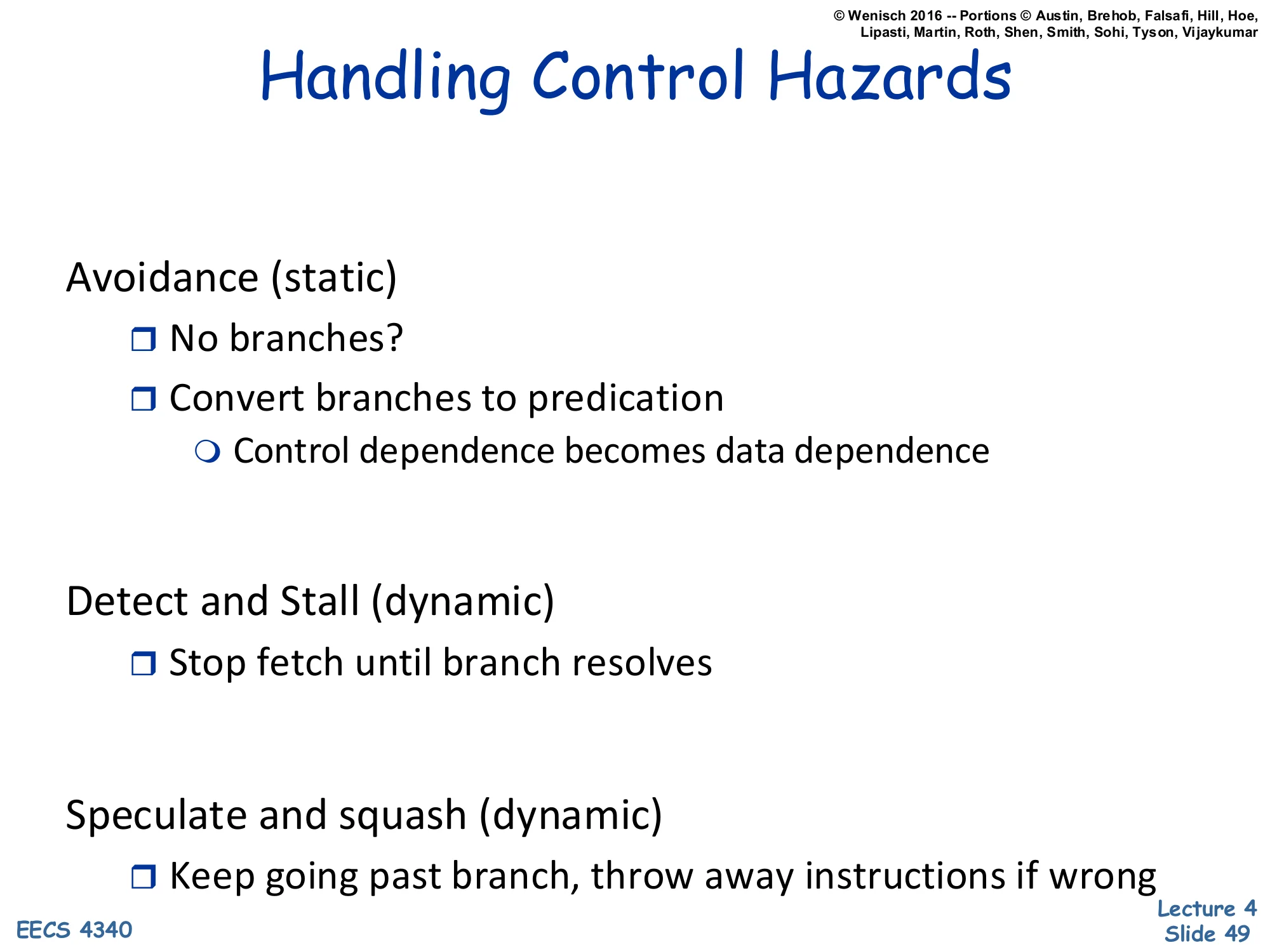
Handling Control Hazards

Avoidance (static)

No branches?
Convert branches to predication
- Control dependence becomes data dependence

Detect and Stall (dynamic)

Stop fetch until branch resolves

Speculate and squash (dynamic)

Keep going past branch, throw away instructions if wrong

The structure mirrors the data-hazard taxonomy: avoidance, detect-and-stall, and speculate-and-squash (the control analogue of forwarding). Avoidance ranges from “don’t have branches” (impractical) to predication — turn the conditional execution into a data dependence by always executing both paths and using a conditional move (cmov) to commit only the correct result. The next slide demonstrates this with if-conversion. Detect-and-stall simply freezes fetch until the branch resolves, costing exactly the branch-resolution depth in stalled cycles per branch (catastrophic for high-branch-density code). Speculate-and-squash keeps fetching past the branch on a guess, then either lets the speculative work commit (right) or throws it away (wrong). Modern CPUs combine speculation with branch prediction to make the guess accurate well over 95% of the time, so the penalty is rarely paid. The lecture covers each in turn over the next several slides.

Avoidance: if-conversion

Show slide text

Avoidance: if-conversion

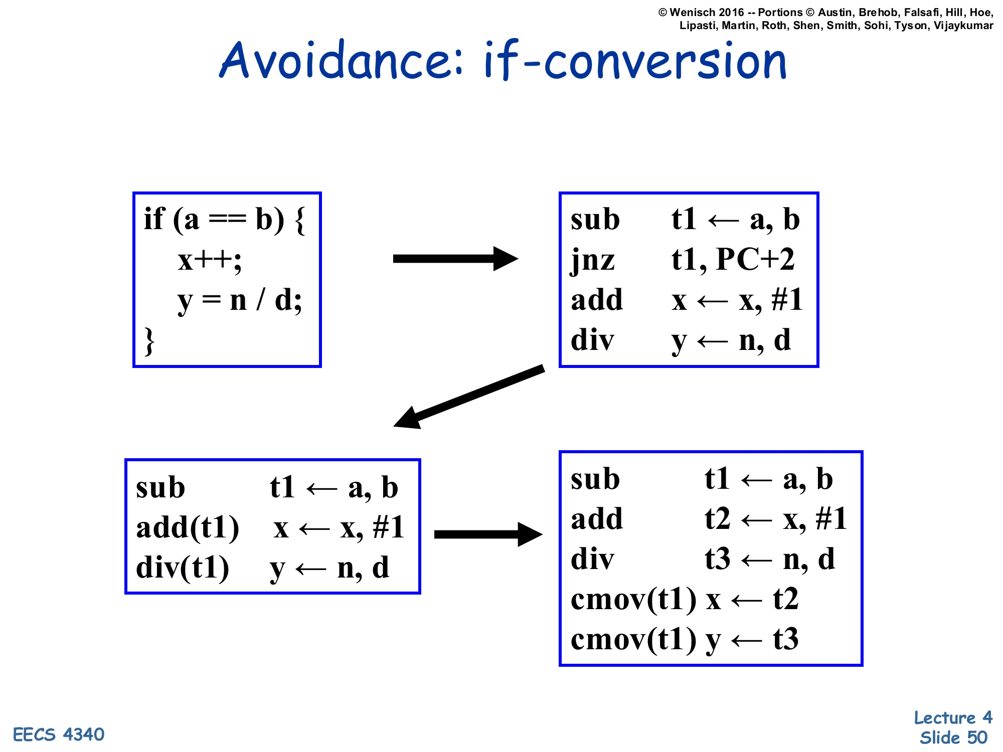
Source:

if (a == b) {
  x++;
  y = n / d;
}

Naïve compiled form (with branch):

sub  t1 ← a, b
jnz  t1, PC+2
add  x ← x, #1
div  y ← n, d

After if-conversion using guarded operations (predicated on t1):

sub      t1 ← a, b
add(t1)  x ← x, #1
div(t1)  y ← n, d

After if-conversion using cmov:

sub       t1 ← a, b
add       t2 ← x, #1
div       t3 ← n, d
cmov(t1)  x  ← t2
cmov(t1)  y  ← t3

If-conversion (a.k.a. predication) eliminates the branch by turning the conditional control flow into a data dependence. The middle form uses guarded instructions (notation add(t1) means “perform the add only if t1 is true”). The bottom form uses unconditional execution followed by a conditional move (cmov(t1) x ← t2 writes t2 into x only if t1 is true). Either way, the pipeline never has to predict or squash anything — both the “taken” and “not-taken” computations always execute, and only their commit depends on the predicate. The ARM ISA generalises this to nearly every instruction (addEQ, subNE, etc.); x86 has cmov for integers and vblend for vectors. The trade-off: predication wastes execution slots when the predicate is biased towards one direction, and it can’t help with loops or backward branches. Compilers reach for if-conversion mostly on small, balanced if/else bodies.

Handling Control Hazards: Detect & Stall

Show slide text

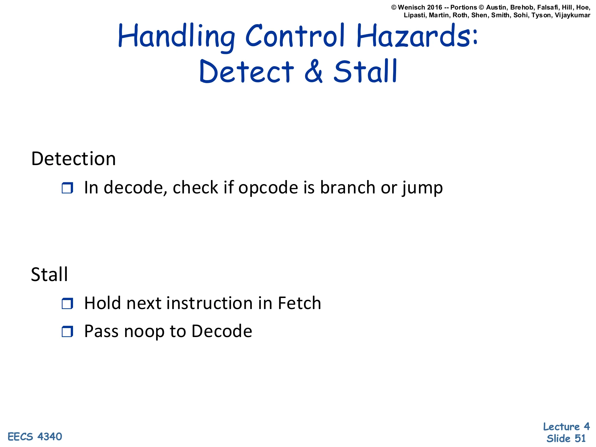
Handling Control Hazards: Detect & Stall

Detection

In decode, check if opcode is branch or jump

Stall

Hold next instruction in Fetch
Pass noop to Decode

The detect-and-stall approach for control hazards mirrors its data-hazard cousin. Detection is trivial: in decode, the opcode field tells you immediately whether the instruction is a branch (e.g. beq) or unconditional jump. Stall action: freeze the PC and IF/ID, and inject a NOP into ID/EX. The pipeline waits until the branch resolves (in EX, one cycle later, when the equality comparator produces its verdict). Once the resolution is known, the PC is steered to the correct target (PC+1 or branch-target). The cost is one cycle of bubble per branch. Programs with high branch density (~20% of instructions for SPEC integer) would lose a fifth of their throughput to this scheme — unacceptable, which is why real designs went straight to speculate-and-squash with prediction.

Problems with Detect & Stall (control)

Show slide text

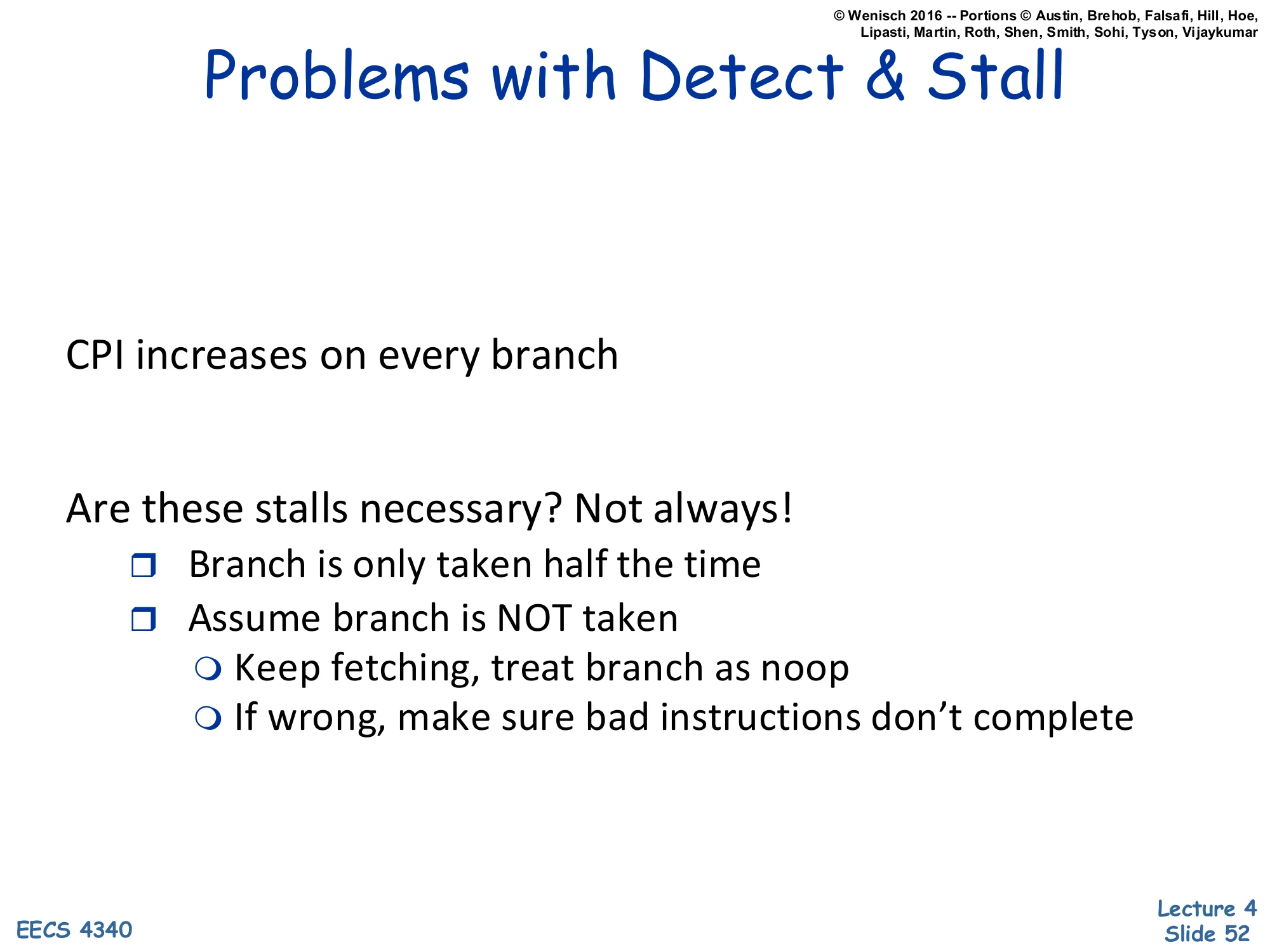
Problems with Detect & Stall

CPI increases on every branch

Are these stalls necessary? Not always!

Branch is only taken half the time
Assume branch is NOT taken
- Keep fetching, treat branch as noop
- If wrong, make sure bad instructions don’t complete

The same critique that motivated forwarding now motivates speculation. Every branch raises CPI under detect-and-stall, but empirically branches are taken roughly half the time (it varies; backward branches in loops are taken ~95% of the time, forward branches near 50%). So a static “assume not taken” policy gets the right answer for free on the not-taken branches and incurs the squash cost only on the taken ones. Pseudocode: keep fetching past the branch as if nothing happened. If the branch resolves not-taken, you win — the in-flight instructions were the right ones and they continue. If it resolves taken, you’ve executed instructions that shouldn’t run; squash them before they update architectural state. This is the speculate-and-squash scheme, formalised on the next slide.

Handling Control Hazards: Speculate & Squash

Show slide text

Handling Control Hazards: Speculate & Squash

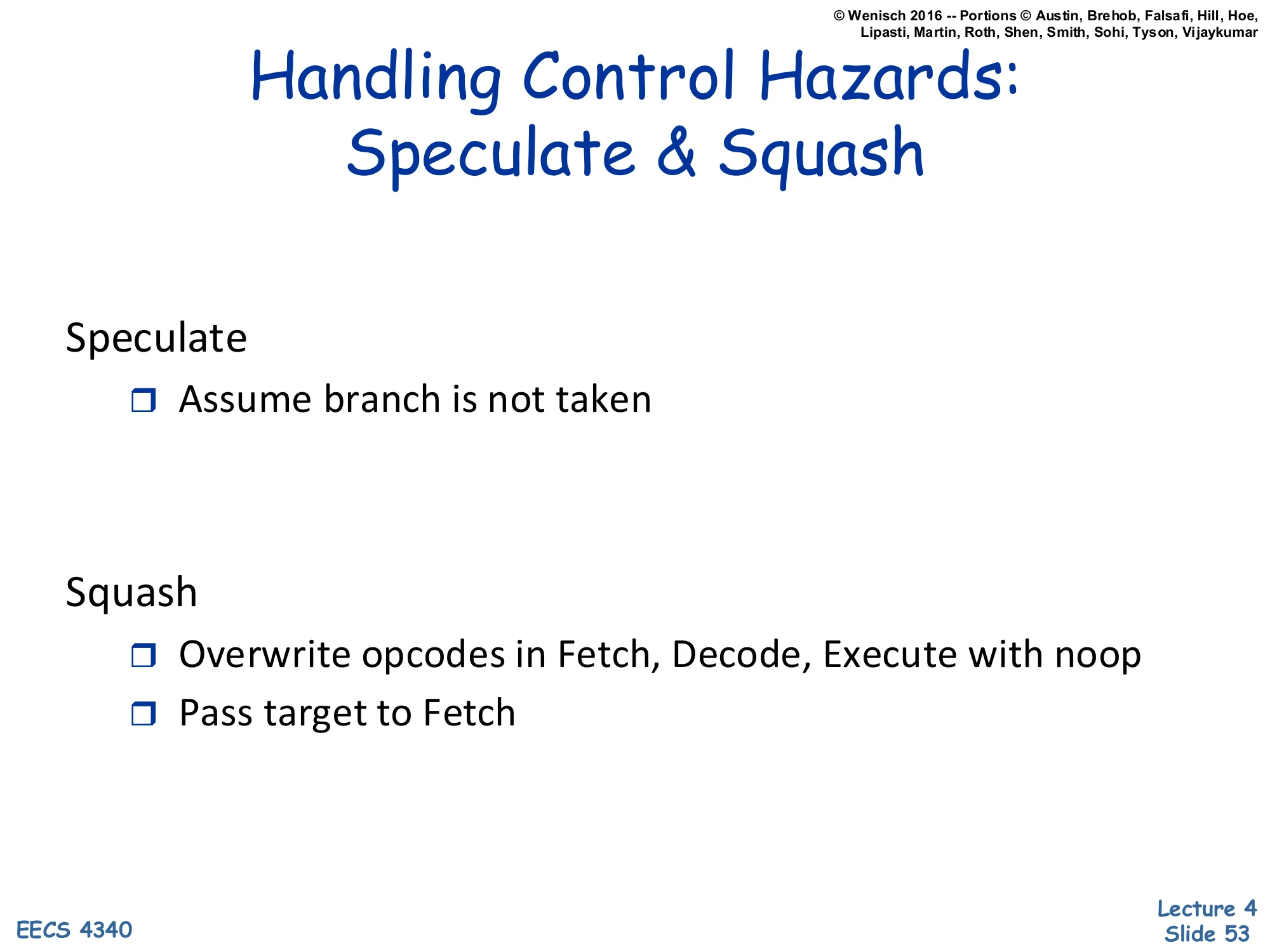
Speculate

Assume branch is not taken

Squash

Overwrite opcodes in Fetch, Decode, Execute with noop
Pass target to Fetch

Speculate-and-squash is the runtime version of “assume not taken”. Speculate: the front end keeps fetching at PC+1 every cycle, even when a branch is in flight, betting that the branch will fall through. Squash on misprediction: when the branch resolves taken (the equality test in EX returns true), the pipeline (i) overwrites every instruction younger than the branch in IF, ID, EX with NOP encodings — they will become harmless bubbles as they advance, (ii) sends the correct target address to the PC for fetch on the next cycle. Crucially, no architectural state has been corrupted because the squashed instructions never reach WB. The next slide shows the datapath modifications needed; the slide after shows why static “assume not taken” is too crude for modern workloads.

Datapath modifications for Speculate & Squash

Show slide text

Datapath modifications for Speculate & Squash

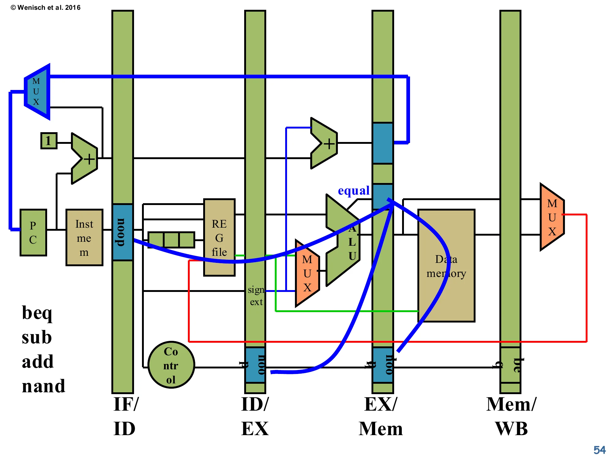
The diagram shows the standard 5-stage datapath with several blue/red overlays:

The equal comparator output in EX/Mem is wired back to the PC MUX as the misprediction signal. When the branch resolves taken, this signal selects the branch-target value (computed by the EX-stage adder) into the PC, redirecting fetch.
Simultaneously, the same misprediction signal forces the opcode fields in IF/ID, ID/EX, and EX/Mem (the slots immediately younger than the branch) to be overwritten with noop — visible as the small blue boxes labelled noop in those latches.
The instruction sequence on the left (beq, sub, add, nand) shows the fetch order; if beq mispredicts, all three trailing instructions are squashed into NOPs.

This is the hardware support for speculate-and-squash. Three changes versus the basic datapath: (1) a new control signal from the branch resolution in EX/Mem feeds back to the IF-stage MUX so a mispredicted-taken branch can redirect fetch immediately to the branch target; (2) the same signal is OR-ed into the opcode-overwrite logic at IF/ID, ID/EX, and EX/Mem so the speculatively-issued instructions are converted to NOPs; (3) the control unit (round node) reads opcodes and decides what to do. The misprediction penalty is the depth at which the branch resolves — three cycles in this 5-stage pipeline, one per squashed instruction. Deeper pipelines suffer proportionally more, which is why deep-pipeline machines like Pentium 4 (20+ stages) leaned heavily on accurate prediction to keep the misprediction rate low.

Problems with Speculate & Squash

Show slide text

Problems with Speculate & Squash

Always assumes branch is not taken

Can we do better? Yes.

Predict branch direction and target!
Why possible? Program behavior repeats.

Branch Delay Slot (MIPS, SPARC)

Show slide text

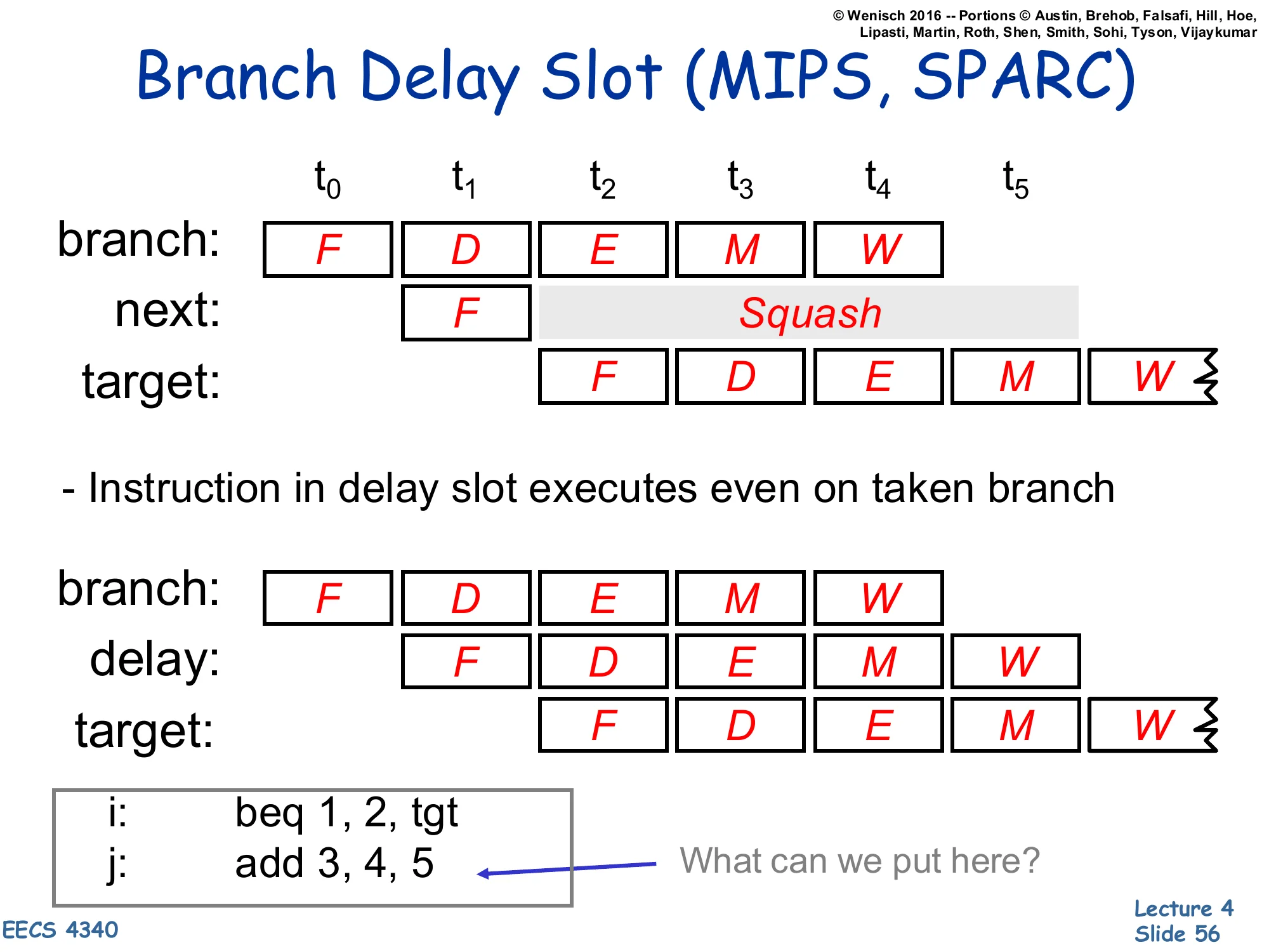
Branch Delay Slot (MIPS, SPARC)

Without delay slot (squash on taken):

Insn	t0	t1	t2	t3	t4	t5
branch	F	D	E	M	W
next		F	Squash	Squash	Squash	Squash
target			F	D	E	M

Instruction in delay slot executes even on taken branch

With delay slot:

Insn	t0	t1	t2	t3	t4	t5
branch	F	D	E	M	W
delay		F	D	E	M	W
target			F	D	E	M

Code example:

i:  beq 1, 2, tgt
j:  add 3, 4, 5     ← What can we put here?

The branch delay slot is the control-hazard analogue of the load delay slot from page 47. MIPS and SPARC both shipped with the architectural rule: “the instruction immediately following a branch is always executed, regardless of whether the branch is taken.” The compiler is then expected to fill the slot with a useful instruction that does no harm in either branch direction (e.g. an unrelated computation), or with a NOP if no such instruction exists. The diagrams contrast: without a delay slot, a taken branch squashes the next instruction; with a delay slot, the next instruction is preserved and runs to completion alongside both possible successor paths. The technique squeezed one extra issue slot out of the early MIPS and SPARC pipelines but, like the load delay slot, broke binary compatibility when later implementations changed pipeline depth and is now considered a historical curiosity. RISC-V dropped it deliberately for that reason.

Pipeline Hazard Checklist

Show slide text

Pipeline Hazard Checklist

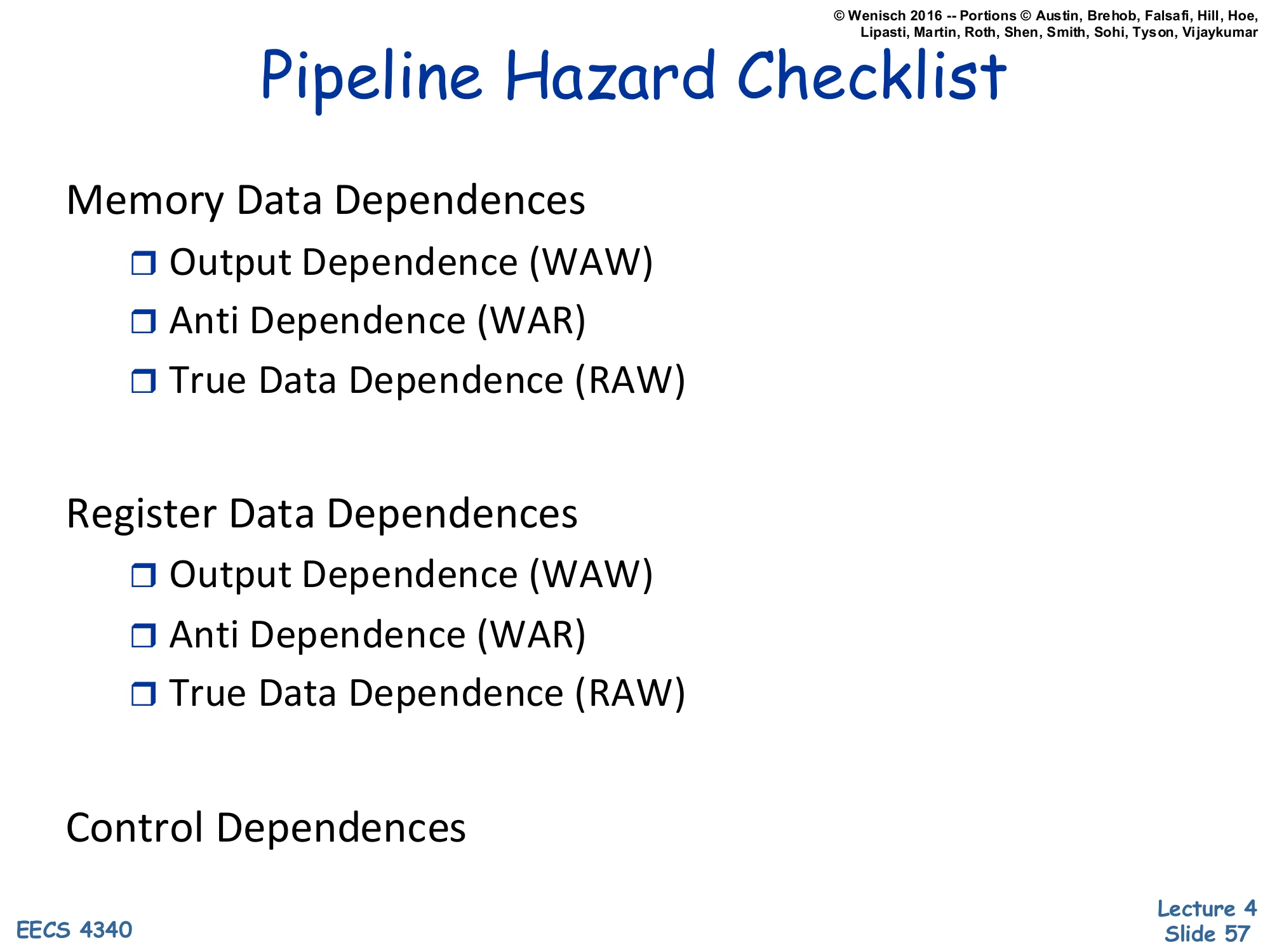
Memory Data Dependences

Output Dependence (WAW)
Anti Dependence (WAR)
True Data Dependence (RAW)

Output Dependence (WAW)
Anti Dependence (WAR)
True Data Dependence (RAW)

Control Dependences

The lecture closes with a checklist that any pipeline design must address. Register data dependences (RAW, WAR, WAW) are the focus of today — only RAW is a real hazard in the in-order 5-stage pipeline, but WAR and WAW will return when out-of-order execution is introduced. Memory data dependences are the same three relations applied to memory locations: a load (memory-RAW) can’t return data older than the youngest store to the same address; a store (memory-WAR or memory-WAW) can’t be reordered past an older store/load to the same address. These are normally enforced by a store buffer and by memory disambiguation hardware in OoO machines. Control dependences are the third category, addressed today by detect-and-stall, predication, or speculate-and-squash with prediction. Future lectures generalise each of these to richer microarchitectures.

Readings

Show slide text

Readings

For today:

H & P Chapter C.1–C.4

For next Tuesday:

H & P Chapter C.5–C.7, 3.1–3.3, 3.10

Announcements

Show slide text

Announcements

Lab #4 this Wednesday
- Please bring your computer
- Involve graded assignments
- Attendance is required and graded
Project #3
- Due: Milestone 18-Feb-26, full 25-Feb-26
Project #4
- Will be released today (16-Feb-26)
- Due: Project proposal 4-Mar-26, Milestone 1 11-Mar-26
- More details in the lab

https://courseworks2.columbia.edu/courses/237081

L04 · Hazards

L04 · Hazards

EECS 4340 · Lecture 4 — Pipelining Hazards

Announcements

Readings

Recap: Pipelining

Outline: Understanding the Execution Core

Pipelining

Time graphs

5-stage datapath

Balancing Pipeline Stages

Balancing Pipeline Stages (Trends)

Pipelining Hazards

The Cost of Deeper Pipelines

Types of Dependencies and Hazards

Terminology

Necessary Conditions for Data Hazards

Handling Data Hazards

Handling Data Hazards: Avoidance

Problems with Avoidance

Handling Data Hazards: Detect & Stall

5-stage datapath (relabelled)

Datapath with Hazard Comparators

End of Cycle 1

End of Cycle 2

First half of cycle 3 — Hazard Detection

Hazard-detection comparator network

Single comparator — gate-level view

First half of cycle 3 — Stall begins

End of cycle 3 — NOP injected

First half of cycle 4 — Hazard still detected

End of cycle 4

First half of cycle 5 — No Hazard

End of cycle 5

Problems with Detect & Stall

Handling Data Hazards: Detect & Forward

paths grows quadratically with machine width

First half of cycle 3 (with forwarding)

End of cycle 3 (forwarding propagated)

First half of cycle 4 — Forward + new hazard

End of cycle 4 (forwarding active)

First half of cycle 5 (cascaded forwarding)

End of cycle 5

First half of cycle 6 — Load-use hazard

End of cycle 6 (load bubble injected)

First half of cycle 7

End of cycle 7

First half of cycle 8 (Mem/WB → ALU forwarding)

End of cycle 8

Load Delay Slot (MIPS R2000)

Control Hazards

Handling Control Hazards

Avoidance: if-conversion

Handling Control Hazards: Detect & Stall

Problems with Detect & Stall (control)

Handling Control Hazards: Speculate & Squash

Datapath modifications for Speculate & Squash

Problems with Speculate & Squash

Branch Delay Slot (MIPS, SPARC)

Pipeline Hazard Checklist

Readings

Announcements