L05 · Scoreboarding

Topic: out-of-order · 53 pages

EECS 4340 Lecture 5 — Scoreboard Scheduling

Announcements

Show slide text

Announcements

No lab this Wednesday
- We will have a lecture instead
Project #3
- Due: 25-Feb-26

https://courseworks2.columbia.edu/courses/237081

Readings

Show slide text

Readings

For today:

H & P Chapter C.5–C.7, 3.1–3.3, 3.10

For Wednesday:

H & P Chapter 3.4–3.6
Design Space of Register Renaming Techniques, https://ieeexplore.ieee.org/abstract/document/877952

Recap: Pipelining Hazards

Outline: Understanding the Execution Core

Show slide text

Outline: Understanding the Execution Core

3827’s 5-stage pipeline (review)
Implementing pipeline interlocks (review)
Scoreboard scheduling (CDC 6600)
Tomasulo’s OoO scheduling algorithm (IBM 360)
Precise interrupts with a Reorder Buffer (P6, Core)
Modern OoO (MIPS R10K, Alpha 21264, Netburst)

This is the multi-week roadmap for the out-of-order portion of EECS 4340. The first two items recap material from L03/L04: the basic five-stage pipeline (3827 is the prerequisite logic-design course code) and the in-order interlock logic that stalls dependent instructions. Items 3–6 trace the historical evolution of dynamic scheduling. Today’s lecture focuses on item 3, scoreboarding — the centralized hardware-tracking scheme introduced in the CDC 6600 (1964). Next lecture covers Tomasulo’s algorithm, which adds register renaming (via reservation stations and the common data bus) to remove the WAR/WAW limitations the scoreboard inherits. After that, a reorder buffer is added to support precise interrupts and speculation (the P6/Core style), and finally the MIPS R10000 / Alpha 21264 / NetBurst style of physical-register-file renaming. Each step removes a limitation of the previous one.

Pipeline Hazard Checklist

Show slide text

Pipeline Hazard Checklist

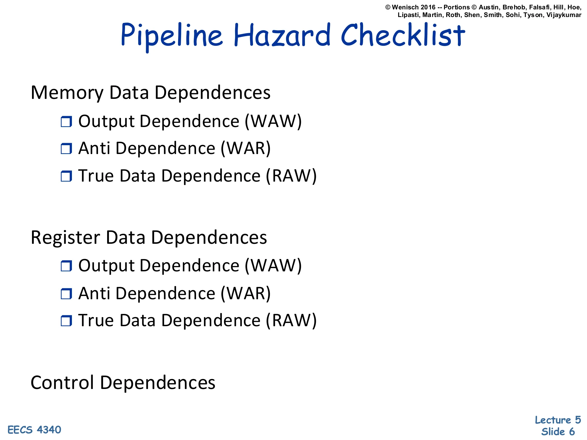
Memory Data Dependences

Output Dependence (WAW)
Anti Dependence (WAR)
True Data Dependence (RAW)

Register Data Dependences

Output Dependence (WAW)
Anti Dependence (WAR)
True Data Dependence (RAW)

Control Dependences

There are three families of pipeline hazards an out-of-order machine must handle. Data hazards come in three flavors: RAW (true dependence) is a real ordering constraint — the consumer needs the producer’s value and cannot proceed without it. WAR (anti-dependence) and WAW (output dependence) are name dependences, not data dependences: they arise only because two instructions happen to use the same architectural register or memory location. They can be eliminated by renaming. The slide deliberately lists data hazards twice — once for memory locations and once for registers — because the disambiguation problem is much harder for memory (you have to compute and compare addresses) than for registers (you can read the architecture’s name field directly). Control hazards arise from branches whose direction or target is not yet known when fetch must continue. Today’s scoreboarding lecture only addresses register data hazards; memory and control are deferred.

Instruction Level Parallelism

ILP: Instruction-Level Parallelism

Show slide text

ILP: Instruction-Level Parallelism

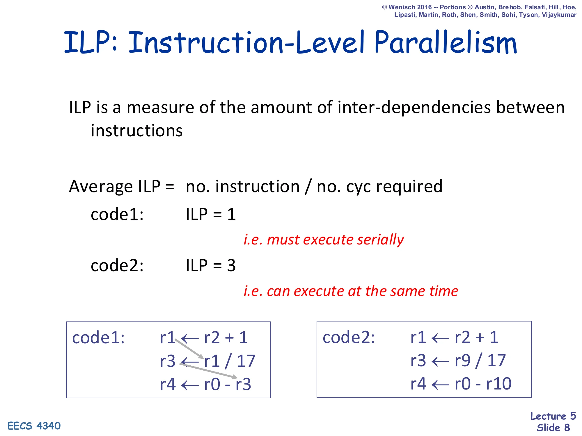
ILP is a measure of the amount of inter-dependencies between instructions.

Average ILP = no. instruction / no. cyc required

code1: ILP = 1 (i.e. must execute serially)
code2: ILP = 3 (i.e. can execute at the same time)

code1:

r1 ← r2 + 1
r3 ← r1 / 17
r4 ← r0 - r3

code2:

r1 ← r2 + 1
r3 ← r9 / 17
r4 ← r0 - r10

Instruction-level parallelism quantifies how many instructions a program could execute in parallel if the hardware were unlimited. The metric is straightforward: $\text{ILP} = \frac{\text{instructions}}{\text{cycles in critical path}}$ . In code1 each instruction reads the previous instruction’s result, so the dependence chain is length 3 and ILP = 3/3 = 1 — the ideal pipeline cannot improve this beyond serial execution because every dependence is a RAW hazard. In code2 the three instructions read disjoint operands and have no inter-dependencies, so all three can execute together: ILP = 3/1 = 3. This number sets the hard ceiling on what any out-of-order machine, no matter how aggressive, can achieve. The job of scoreboarding (and later Tomasulo and renaming) is to expose the available ILP that an in-order pipeline cannot exploit because of false dependencies and rigid issue order.

Purported Limits on ILP

Show slide text

Purported Limits on ILP

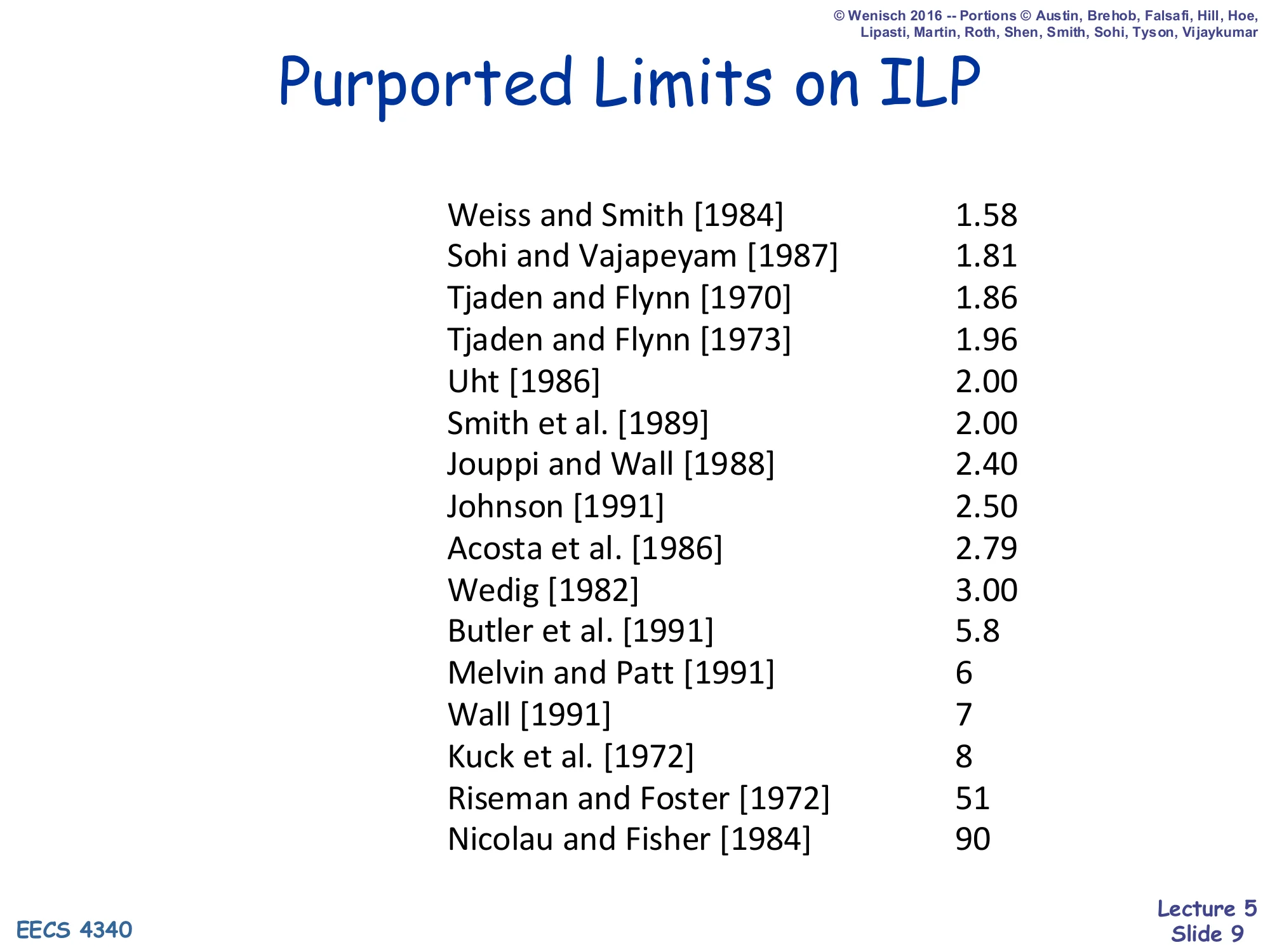
Study	Limit
Weiss and Smith [1984]	1.58
Sohi and Vajapeyam [1987]	1.81
Tjaden and Flynn [1970]	1.86
Tjaden and Flynn [1973]	1.96
Uht [1986]	2.00
Smith et al. [1989]	2.00
Jouppi and Wall [1988]	2.40
Johnson [1991]	2.50
Acosta et al. [1986]	2.79
Wedig [1982]	3.00
Butler et al. [1991]	5.8
Melvin and Patt [1991]	6
Wall [1991]	7
Kuck et al. [1972]	8
Riseman and Foster [1972]	51
Nicolau and Fisher [1984]	90

Two decades of academic studies disagreed wildly about how much ILP is actually available in real programs. The low estimates (1.5–3) come from studies that constrained themselves to small basic blocks, finite issue windows, and realistic branch prediction; the high estimates (51, 90) come from studies that assumed perfect branch prediction, infinite registers, and unlimited reordering across whole loops or programs. The point of this slide is not that one number is right — it is that available ILP depends enormously on the hardware budget you allow. If you give the machine a big enough instruction window, perfect renaming, and a perfect branch predictor, programs really do contain a lot of parallelism. The architectural decisions in the rest of this course (how big a window, what predictor, what renaming style) determine where on this spectrum a real machine lands.

Architectures for ILP — Scalar Pipeline

Show slide text

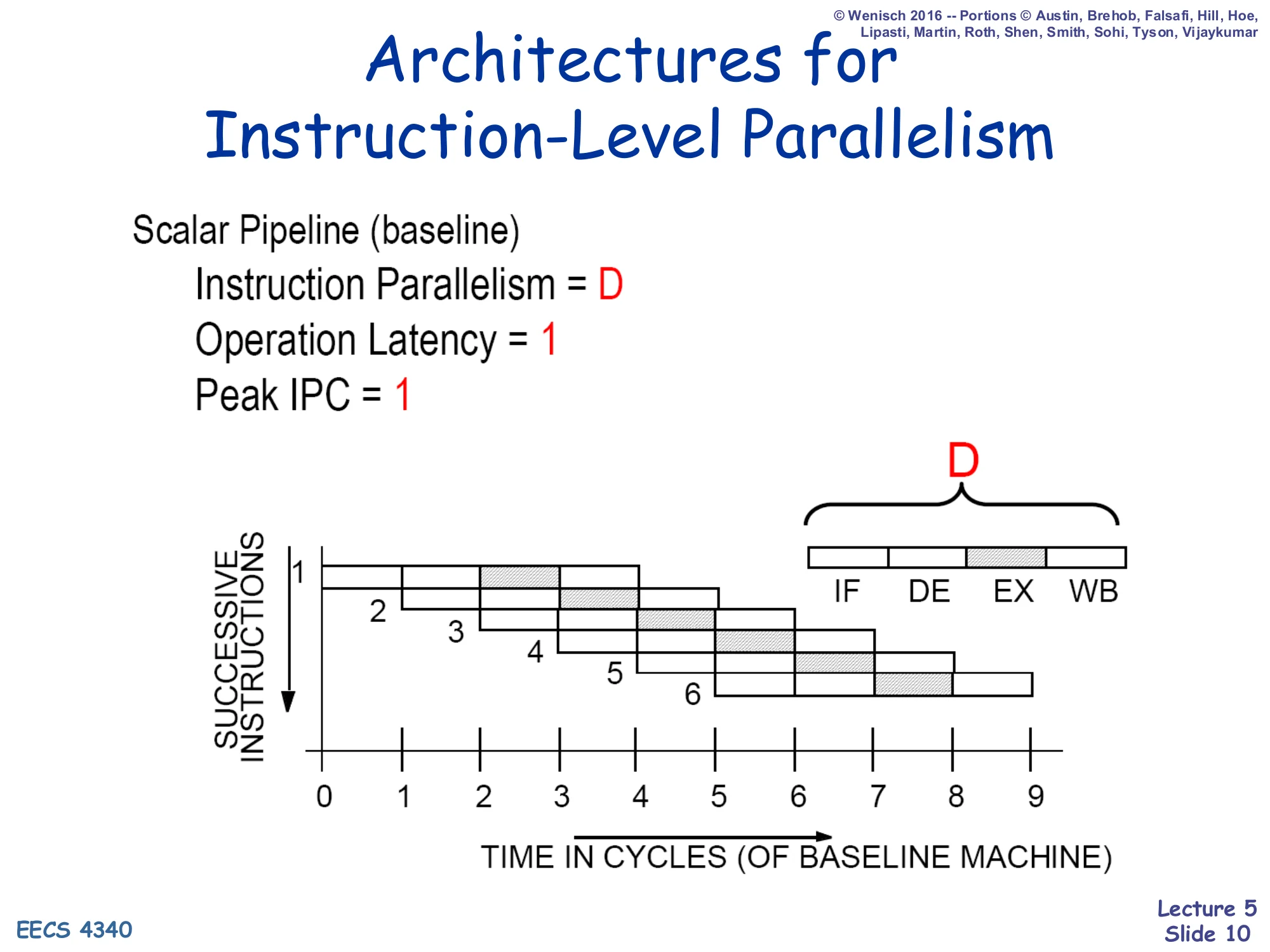
Architectures for Instruction-Level Parallelism

Scalar Pipeline (baseline)

Instruction Parallelism = $D$
Operation Latency = 1
Peak IPC = 1

Diagram: $D$ stages (IF, DE, EX, WB) — each cycle one new instruction enters; up to $D$ instructions are in flight at once.

A scalar in-order pipeline of depth $D$ has, at steady state, $D$ instructions in flight — one in each stage. That is what “instruction parallelism = $D$ ” means here: it is spatial concurrency across stages, not concurrent issue. The peak IPC is still 1 because only one instruction can advance through each stage per cycle. Operation latency is 1 baseline cycle in the sense that each individual operation finishes one cycle after it issues. The picture (six successive instructions overlapping diagonally) is the classic Patterson-style pipeline diagram. This is the floor against which we will measure the value of out-of-order execution. The next slides argue that scalar pipelines have hard ceilings and that a superscalar in-order pipeline does not really fix them.

Limitations of Scalar Pipelines

Show slide text

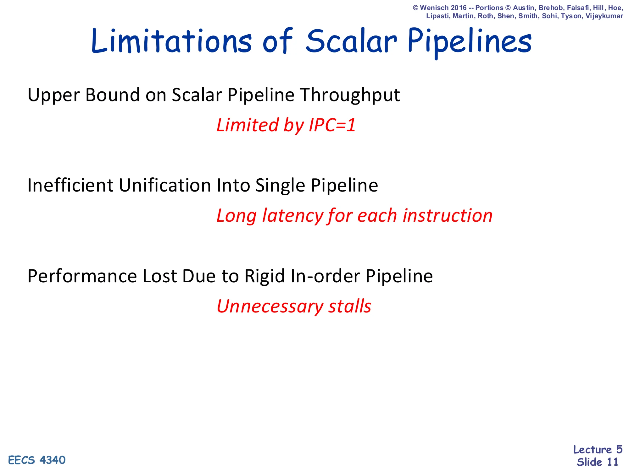
Limitations of Scalar Pipelines

Upper Bound on Scalar Pipeline Throughput — Limited by IPC=1
Inefficient Unification Into Single Pipeline — Long latency for each instruction
Performance Lost Due to Rigid In-order Pipeline — Unnecessary stalls

Three limits motivate everything that follows. First, throughput is capped at one instruction per cycle, so you cannot do better than IPC=1 no matter how fast your clock — the only way past this is multiple-issue (superscalar). Second, forcing every instruction through the same pipeline means a 1-cycle add and a 20-cycle divide share the same latency budget; this is why real machines have multiple, differently sized functional units. Third, even with multiple units, an in-order pipeline serializes instructions that could otherwise run in parallel: a long-latency operation behind a young instruction blocks every younger instruction even when those younger instructions are independent. The third limitation is the one this lecture attacks: dynamic scheduling, beginning with scoreboarding, lets younger independent instructions “pass” older stalled ones.

Superscalar Machine

Show slide text

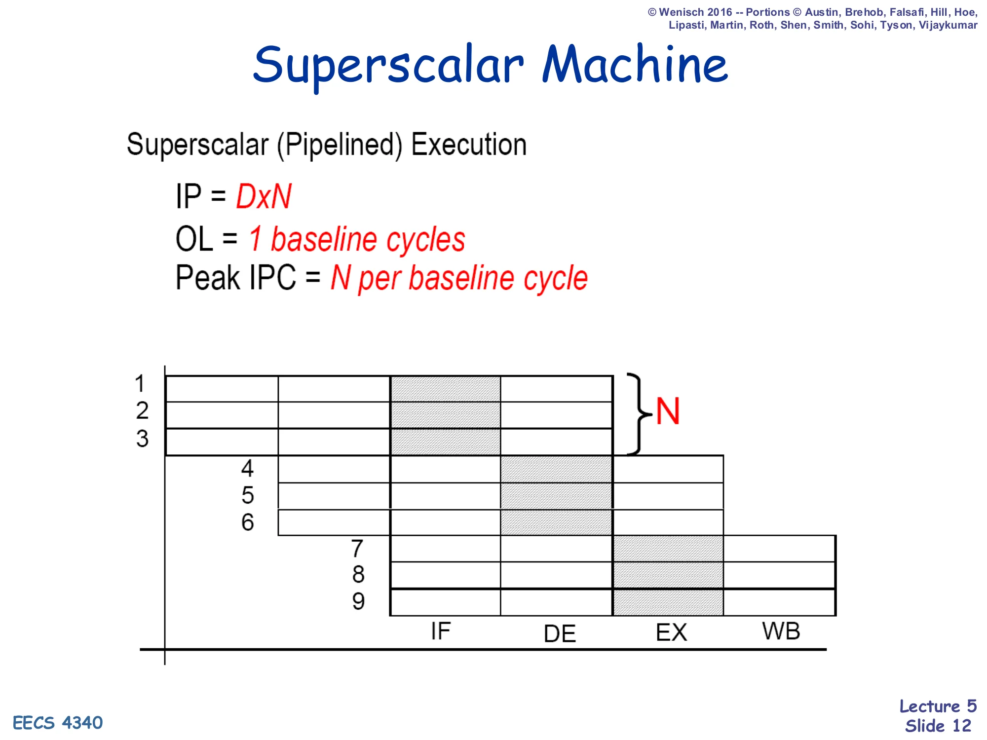
Superscalar Machine

Superscalar (Pipelined) Execution

$\text{IP} = D \times N$
$\text{OL} = 1$ baseline cycle
Peak $\text{IPC} = N$ per baseline cycle

Diagram: $N$ instructions enter every cycle; pipeline width is $N$ , depth is $D$ .

A superscalar of width $N$ replicates each pipeline stage $N$ times so that $N$ independent instructions can advance per cycle. The peak IPC becomes $N$ and the total in-flight count becomes $D \times N$ . This is the standard answer to “throughput is capped at IPC = 1” — issue more instructions per cycle. The figure shows three instructions per cycle entering F, then D, then EX, etc. In an in-order superscalar, a stall of any one instruction in a bundle stalls the whole bundle, so true parallelism still requires either compiler-side scheduling (VLIW/EPIC) or hardware dynamic scheduling. The next slide explains why the in-order version of the superscalar is not enough — and that is what motivates the scoreboard.

What is the real problem?

Show slide text

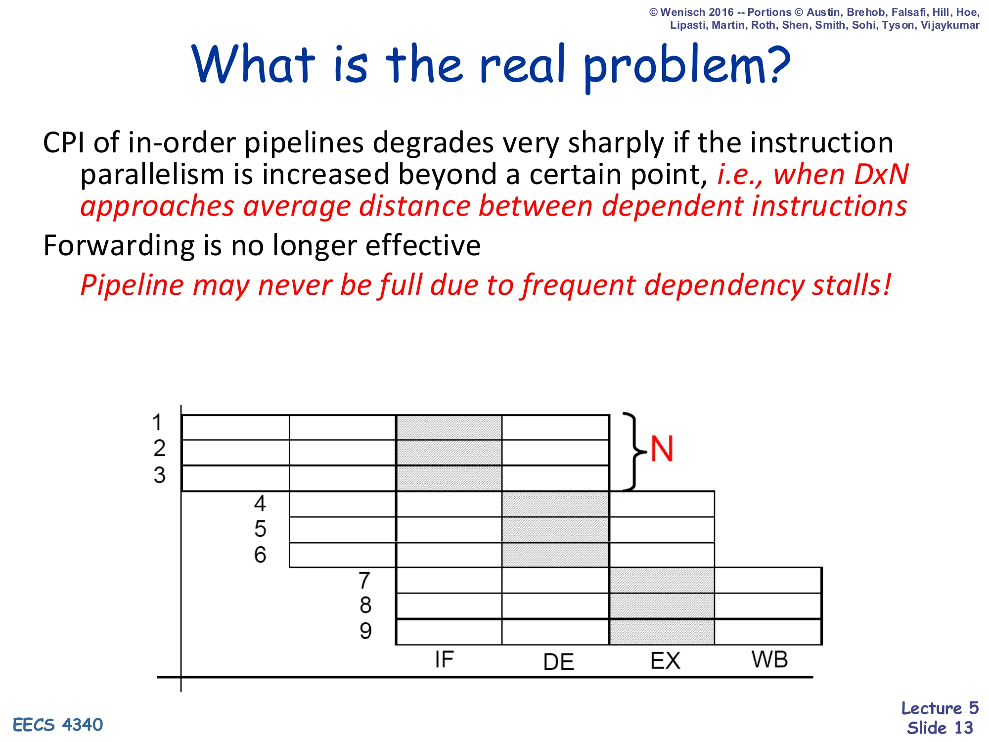
What is the real problem?

CPI of in-order pipelines degrades very sharply if the instruction parallelism is increased beyond a certain point, i.e., when $D \times N$ approaches average distance between dependent instructions.

Forwarding is no longer effective.

Pipeline may never be full due to frequent dependency stalls!

As you make a pipeline wider ( $N$ ) and/or deeper ( $D$ ), the product $D \times N$ — the number of in-flight instructions — eventually exceeds the average distance between dependent instructions in the program. Once that happens, almost every issued instruction is waiting on an in-flight result, forwarding cannot bridge the gap any more (because forwarding only collapses one or two stages), and CPI degrades sharply. The pipeline diagram on the slide shows exactly this: nine instructions are in flight but the back of the pipeline is sitting idle waiting on RAW dependencies in the front. In-order execution cannot recover this lost work. To fill that idle space the hardware must look past the stalled instruction and find an independent younger instruction to issue — that is dynamic scheduling, and the rest of this lecture builds the simplest version of it.

Necessary Conditions for Data Hazards

Show slide text

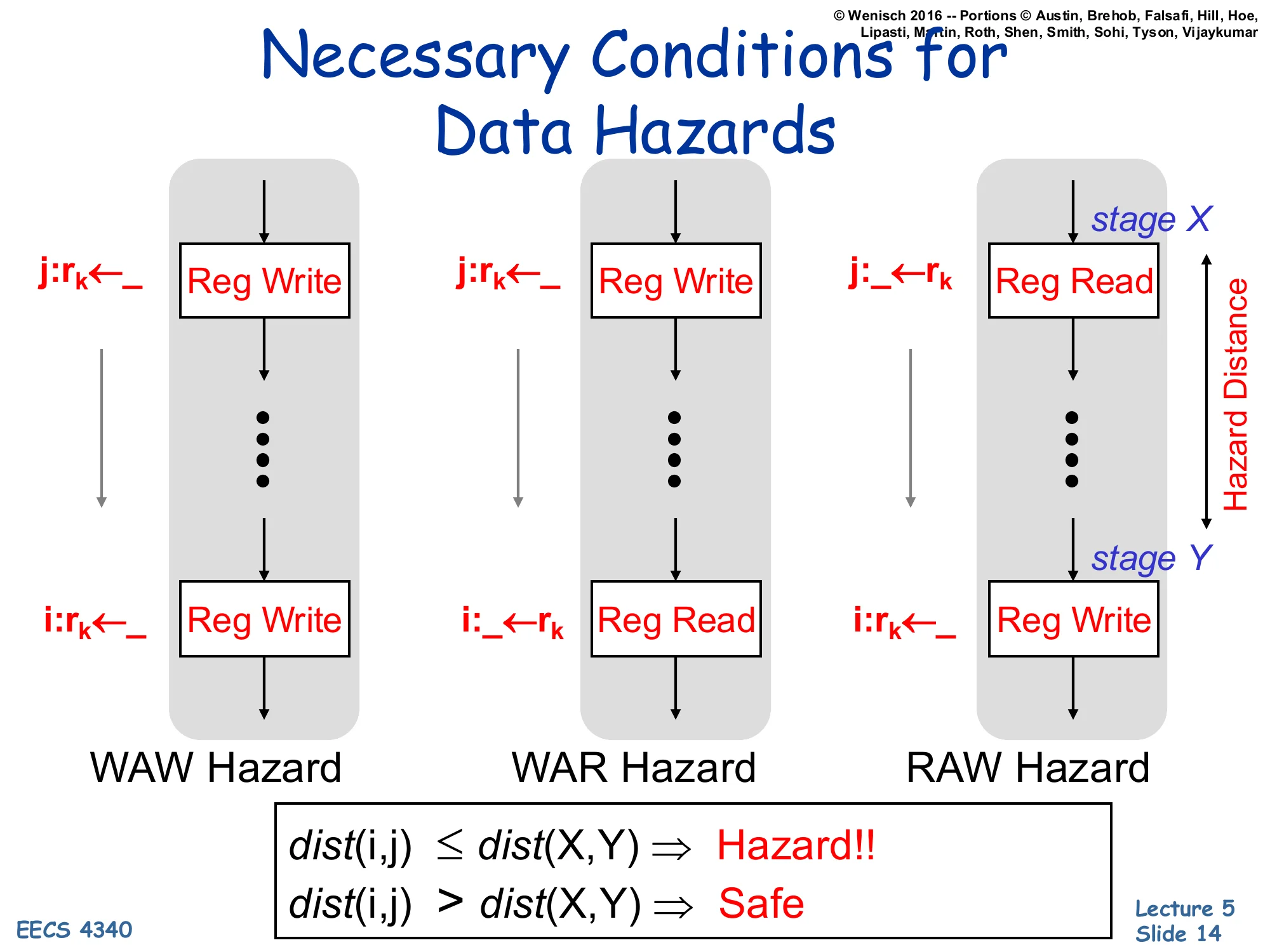
Necessary Conditions for Data Hazards

For each hazard kind, the producer/consumer pair touches the same register $r_k$ at two specific stages (Reg Write or Reg Read), and the hazard distance between those two stages must be at least the instruction distance between $i$ and $j$ :

WAW Hazard: $j: r_k \leftarrow \_$ (Reg Write) … $i: r_k \leftarrow \_$ (Reg Write)
WAR Hazard: $j: r_k \leftarrow \_$ (Reg Write) … $i: \_ \leftarrow r_k$ (Reg Read)
RAW Hazard: $j: \_ \leftarrow r_k$ (Reg Read at stage X) … $i: r_k \leftarrow \_$ (Reg Write at stage Y)

$\text{dist}(i,j) \le \text{dist}(X,Y) \Rightarrow \text{Hazard!!}$

$\text{dist}(i,j) > \text{dist}(X,Y) \Rightarrow \text{Safe}$

A hazard exists only when two conditions both hold: the two instructions name the same register, and they are close enough together that the older one has not yet finished by the time the younger one needs it. The slide formalizes this as the comparison $\text{dist}(i,j) \le \text{dist}(X,Y)$ , where $\text{dist}(i,j)$ is the program-order gap between the two instructions and $\text{dist}(X,Y)$ is the gap between the producing and consuming pipeline stages. For example, if RAW reads happen in stage 2 and writes in stage 5, the hazard distance is 3 cycles — any consumer fewer than 3 instructions behind the producer will stall. This way of thinking pays off later: a RAW hazard is intrinsic (you actually need the value) but a WAR or WAW is purely an artifact of when writes happen relative to reads, so reordering the writes (via renaming) makes them disappear.

Class Task — Identify Hazards

Show slide text

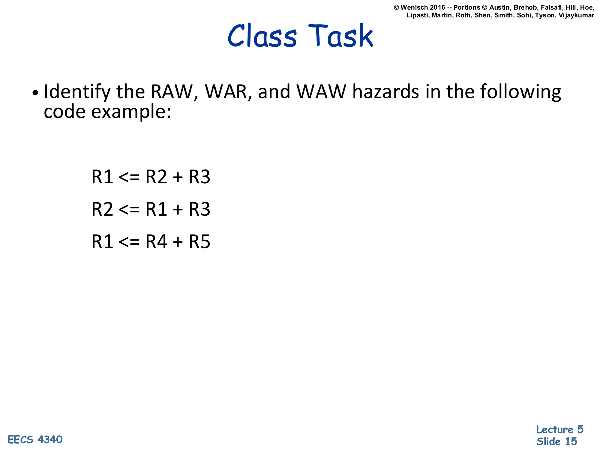
Class Task

Identify the RAW, WAR, and WAW hazards in the following code example:

R1 <= R2 + R3
R2 <= R1 + R3
R1 <= R4 + R5

Walking through the three-instruction snippet: instruction 2 reads R1, which instruction 1 just wrote — that is a RAW on R1 between insns 1→2. Instruction 2 writes R2, which instruction 1 read — that is a WAR on R2 between insns 1→2. Instruction 3 writes R1, which instruction 1 also wrote — that is a WAW on R1 between insns 1→3. There is also a WAR on R1 between insns 2 (reads R1) and 3 (writes R1). The RAW is the only real dependency: instruction 2 genuinely needs the result of instruction 1. Both the WAR and the WAW are name conflicts: if you rename instruction 3’s destination to a different physical register (and propagate the name change to any consumer that read the old R1), insns 1 and 3 can run in parallel. This is the central insight that justifies register renaming in Tomasulo and beyond.

The Problem With In-Order Pipelines

Show slide text

The Problem With In-Order Pipelines

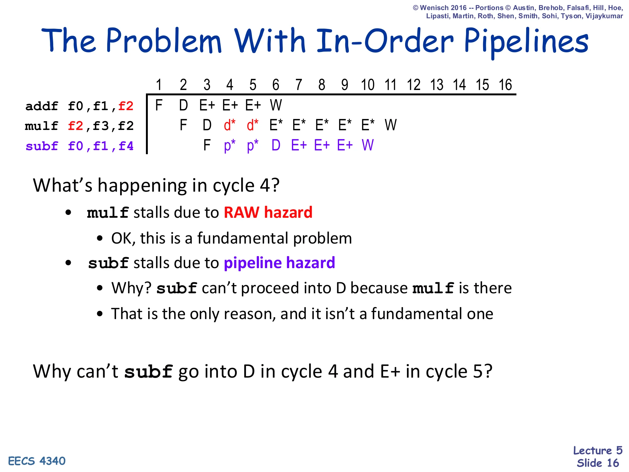
               1  2  3  4  5  6  7  8  9 10 11 12 ...
addf f0,f1,f2  F  D  E+ E+ E+ W
mulf f2,f3,f2     F  D  d* d* E* E* E* E* E* W
subf f0,f1,f4        F  p* p* D  E+ E+ E+ W

What’s happening in cycle 4?

mulf stalls due to RAW hazard — OK, this is a fundamental problem
subf stalls due to pipeline hazard
- Why? subf can’t proceed into D because mulf is there
- That is the only reason, and it isn’t a fundamental one

Why can’t subf go into D in cycle 4 and E+ in cycle 5?

This pipeline diagram is the exact motivation for dynamic scheduling. The mulf legitimately stalls — it has a RAW on f2 from the preceding addf, and there is nothing the hardware can do about that real data dependency. But the subf underneath stalls only because the in-order machine cannot let it pass the stuck mulf: subf reads f0 and f1 (already ready) and writes f4 (no conflict). It is fully ready to execute in cycle 5, but the rigid in-order discipline blocks decode behind the stalled mulf. The label p* in the diagram is a “pipeline hazard” stall — a structural stall that exists only because of the in-order pipeline organization, not because of any real dependency. Letting subf issue ahead of mulf would recover those wasted cycles. That capability is exactly what a scoreboard provides.

Dynamic Scheduling: The Big Picture

Show slide text

Dynamic Scheduling: The Big Picture

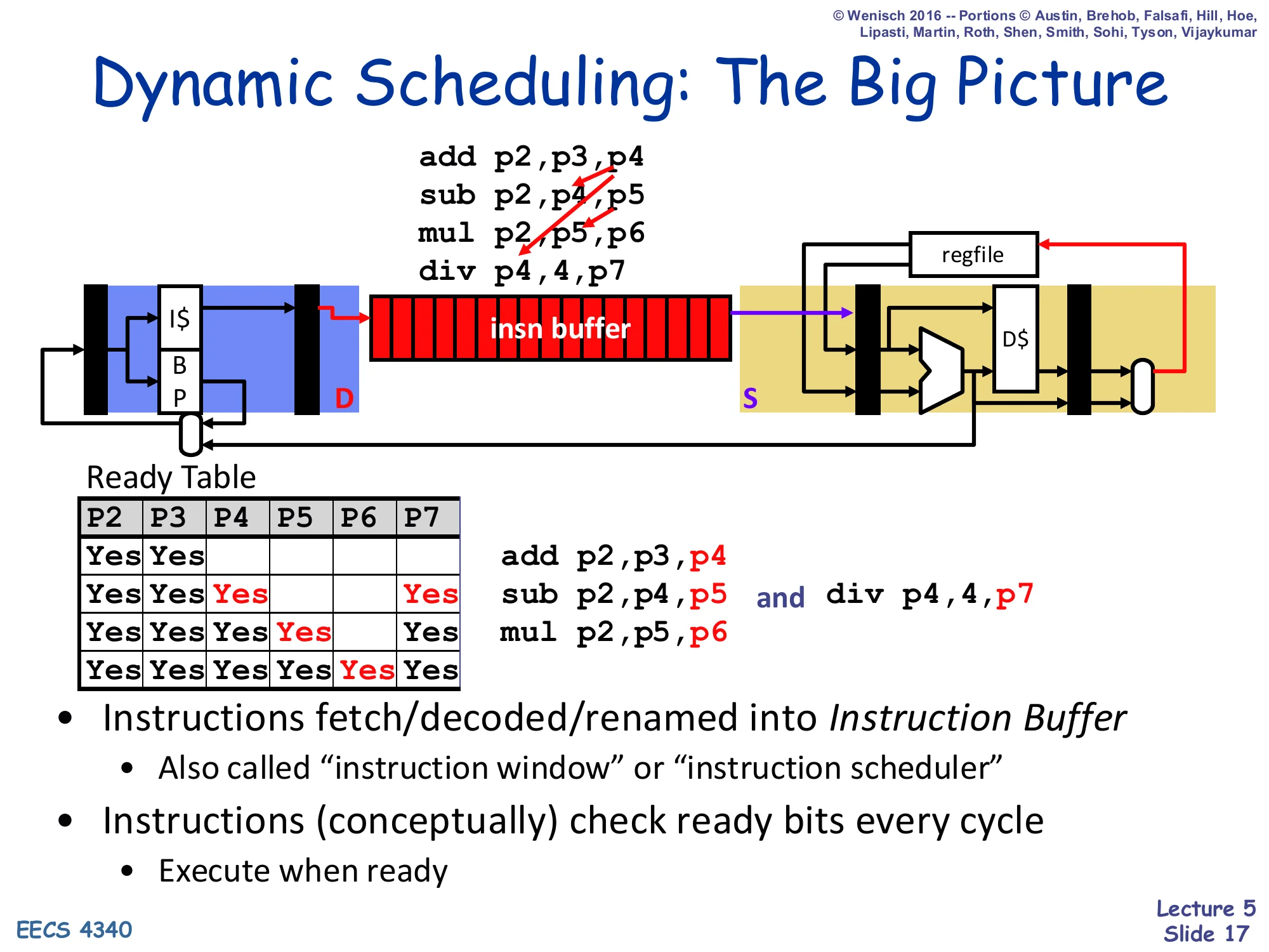
Front-end fetches/decodes/renames instructions into an Instruction Buffer (IB), then they wait until ready and issue out-of-order to the execution units, results write back to the register file.

Example renamed sequence:

add p2,p3,p4
sub p2,p5,p5
mul p2,p5,p6
div p4,4,p7

Ready Table (per physical register: ready-bit):

	P2	P3	P4	P5	P7
t0	Yes	Yes
t1	Yes	Yes	Yes		Yes
t2	Yes	Yes	Yes	Yes
t3	Yes	Yes	Yes	Yes

Instructions fetch/decoded/renamed into Instruction Buffer
- Also called “instruction window” or “instruction scheduler”
Instructions (conceptually) check ready bits every cycle
- Execute when ready

This slide is a preview of the entire OoO front-end/back-end split. Instructions are fetched in program order, decoded, and renamed (architectural register names mapped to physical-register names like p2, p3, …). The renamed instructions are dropped into a many-entry instruction buffer (also called the instruction window or scheduler) and wait there. Each cycle the scheduler scans the buffer and fires any instruction whose physical-register source operands have all been produced — that is what the per-physical-register “Ready Table” captures. The example shows that after rename, sub p2,p5,p5 and div p4,4,p7 both become ready as soon as their operands appear, even though they are not adjacent in program order. The picture at the top of the slide foreshadows Tomasulo — the scoreboard we are about to build is a much simpler version of this idea that does not yet rename.

Register Renaming

Show slide text

Register Renaming

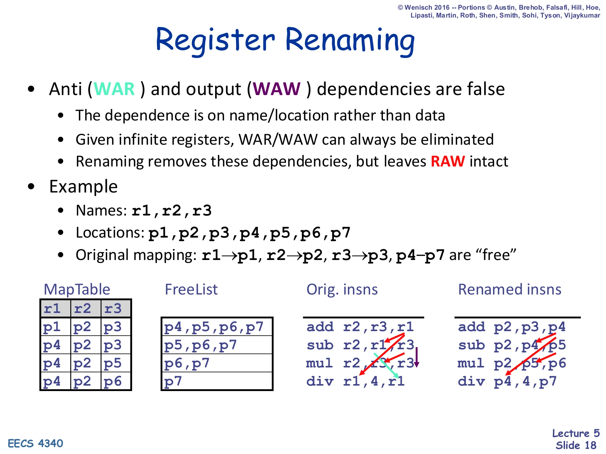
Anti (WAR) and output (WAW) dependencies are false
- The dependence is on name/location rather than data
- Given infinite registers, WAR/WAW can always be eliminated
- Renaming removes these dependencies, but leaves RAW intact
Example
- Names: r1, r2, r3
- Locations: p1, p2, p3, p4, p5, p6, p7
- Original mapping: r1→p1, r2→p2, r3→p3, p4–p7 are “free”

MapTable r1 r2 r3	FreeList	Orig. insns	Renamed insns
p1 p2 p3	p4,p5,p6,p7	add r2,r3,r1	add p2,p3,p4
p4 p2 p3	p5,p6,p7	sub r1,r2,r3	sub p4,p2,p3 (note: r1 reads new p4)
p4 p2 p5	p6,p7	mul r2,r1,r3	mul p2,p4,p5
p4 p2 p6	p7	div r1,4,r1	div p4,4,p7

Register renaming is the systematic mechanism for removing WAR and WAW hazards. Each architectural-register write is given a fresh physical-register name from a free list, and every later read of that same architectural register is mapped through the map table to the new physical name. After renaming, no two in-flight instructions write the same physical register (eliminating WAW) and no in-flight write conflicts with an in-flight read of the prior version (eliminating WAR). RAW dependences survive renaming because they describe real data flow: a consumer must wait for the physical register the producer is writing. The example walks through four instructions; notice how r1 cycles through three different physical names (p1, p4, p7) as it is repeatedly written, and how each consumer reads whichever physical version was the live one at decode time. This is the renaming engine that Tomasulo supplies but the scoreboard does not.

Dynamic Scheduling — OoO Execution

Show slide text

Dynamic Scheduling — OoO Execution

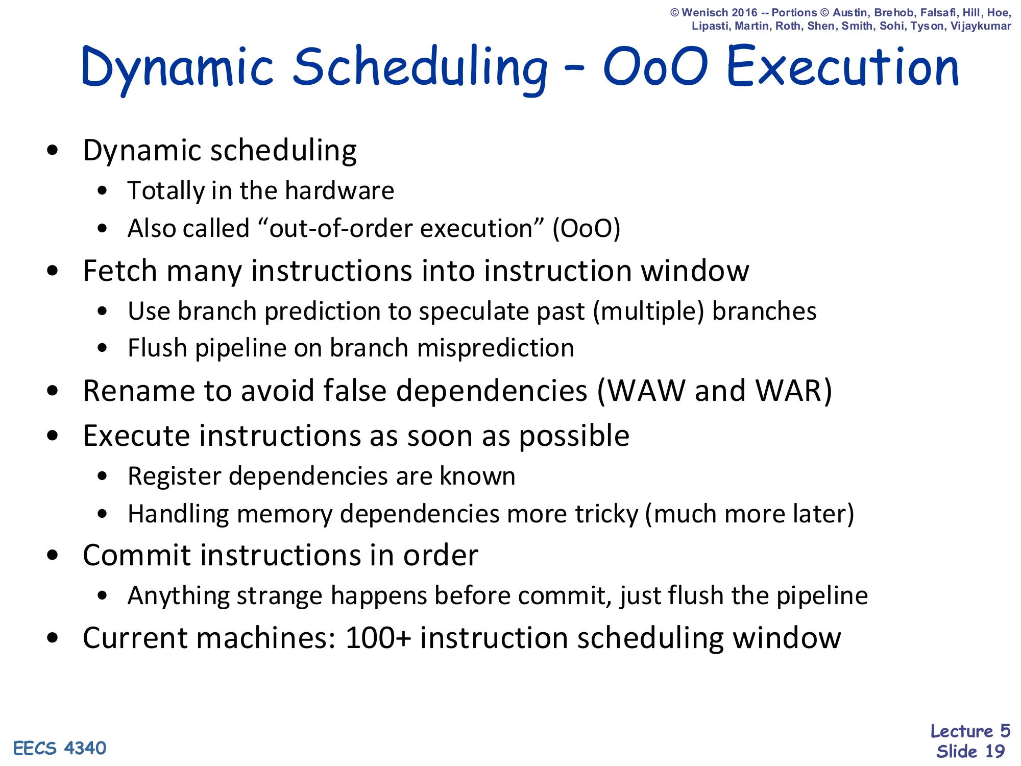
Dynamic scheduling
- Totally in the hardware
- Also called “out-of-order execution” (OoO)
Fetch many instructions into instruction window
- Use branch prediction to speculate past (multiple) branches
- Flush pipeline on branch misprediction
Rename to avoid false dependencies (WAW and WAR)
Execute instructions as soon as possible
- Register dependencies are known
- Handling memory dependencies more tricky (much more later)
Commit instructions in order
- Anything strange happens before commit, just flush the pipeline
Current machines: 100+ instruction scheduling window

This slide is the executive summary of every modern out-of-order core. The hardware fetches and decodes deep into the program — past unresolved branches, using branch prediction to keep the front end busy — and accumulates instructions in a large window (100+ entries on current chips). Inside the window, hardware renaming removes WAR/WAW false dependencies, and instructions execute as soon as their RAW operands arrive, in any order. To preserve sequential semantics and to support precise interrupts, instructions commit in program order using a reorder buffer: if anything goes wrong (mispredicted branch, exception, memory ordering violation), every in-flight younger instruction is squashed and the architectural state is rolled back to the last committed point. Memory dependencies are intentionally hand-waved here because they cannot be fully resolved at rename — addresses are not known until the load/store executes.

Motivation for Dynamic Scheduling

Show slide text

Motivation for Dynamic Scheduling

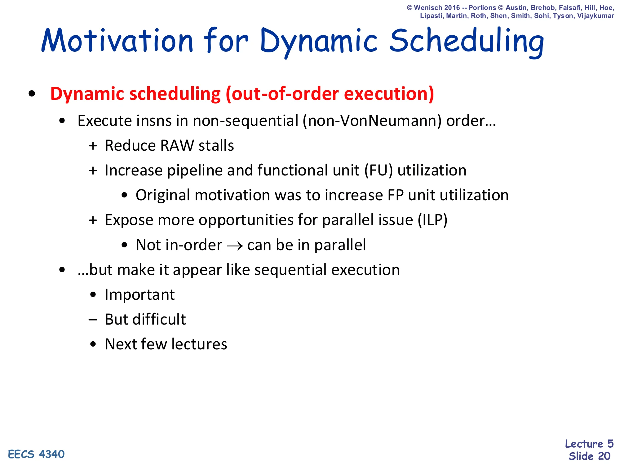
Dynamic scheduling (out-of-order execution)
- Execute insns in non-sequential (non-VonNeumann) order…
- $+$ Reduce RAW stalls
- $+$ $+$ Increase pipeline and functional unit (FU) utilization
  - Original motivation was to increase FP unit utilization
- $+$ $+$ Expose more opportunities for parallel issue (ILP)
  - Not in-order $\rightarrow$ can be in parallel
…but make it appear like sequential execution
- Important
- But difficult
- Next few lectures

Dynamic scheduling — executing instructions in a non-sequential order chosen by hardware — is a tradeoff. The benefits are real: it reduces RAW stalls (younger independent instructions can run while an older one waits), it keeps long-latency functional units (especially FP units) busy, and it exposes ILP that an in-order pipeline cannot reach. The historical context is worth keeping in mind: Tomasulo’s original motivation (IBM 360/91, 1967) was that the FP add and FP multiply units would otherwise sit idle because of dependencies in scientific code. The catch is the words “but make it appear like sequential execution”: software was written assuming Von Neumann sequential semantics, so no matter what order the hardware actually executes things in, exceptions and externally visible state must look like the architecturally specified order. This requirement is what drives the reorder buffer and in-order commit mechanisms in later lectures.

Going Forward: What's Next

Show slide text

Going Forward: What’s Next

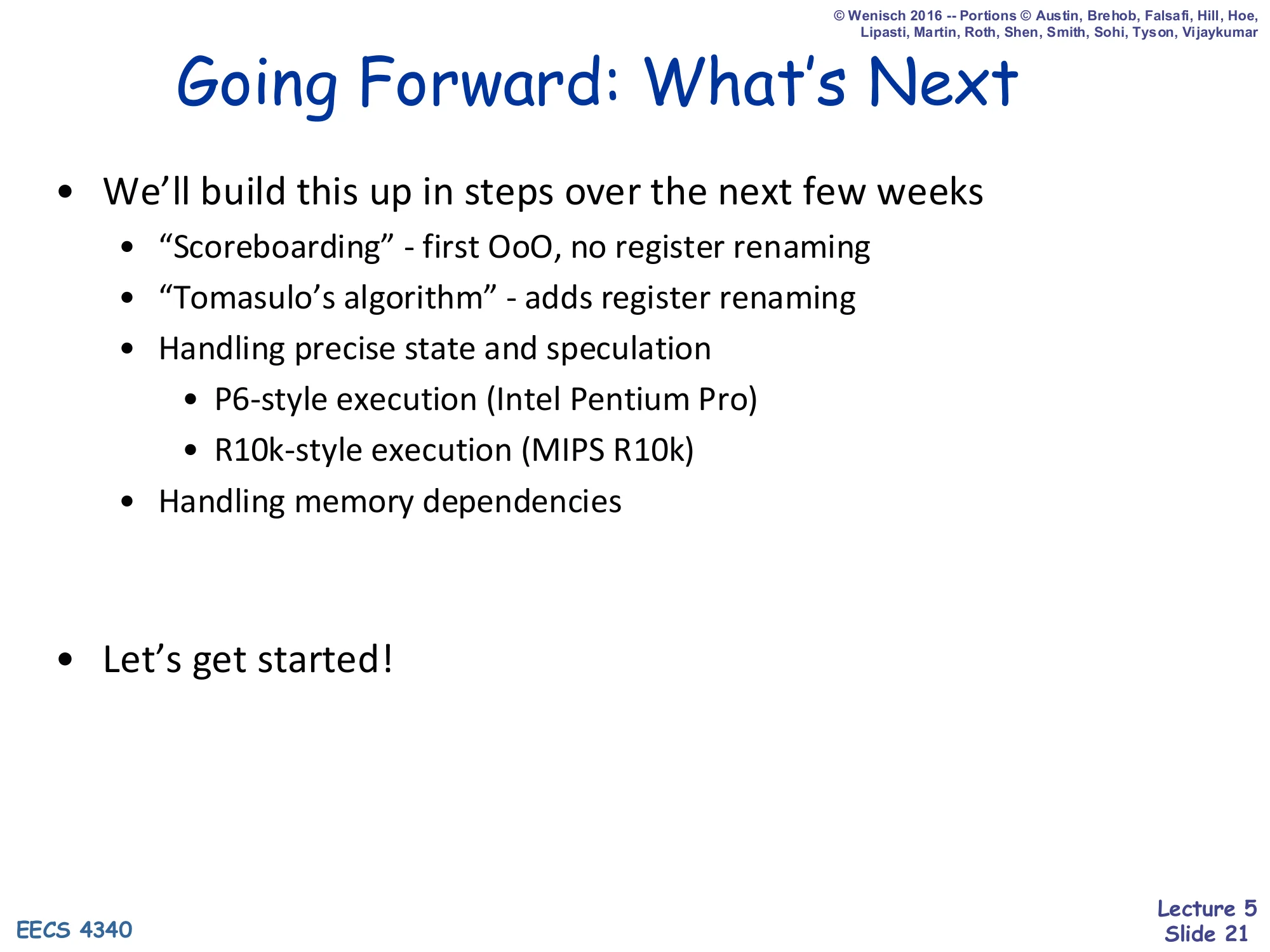
We’ll build this up in steps over the next few weeks
- “Scoreboarding” — first OoO, no register renaming
- “Tomasulo’s algorithm” — adds register renaming
- Handling precise state and speculation
  - P6-style execution (Intel Pentium Pro)
  - R10k-style execution (MIPS R10k)
- Handling memory dependencies
Let’s get started!

A more concrete view of the same roadmap. Scoreboarding (the CDC 6600 design from 1964) is the first hardware out-of-order scheme; it supplies the centralized status table but does no renaming, so it pays a real price for WAR and WAW hazards. Tomasulo (IBM 360/91, 1967) adds renaming via reservation stations and a common data bus but does not yet handle precise interrupts — exceptions in the original Tomasulo machine were imprecise. P6-style (Intel Pentium Pro / Core) and R10K-style (MIPS R10000) machines fix that with two different approaches to combining a reorder buffer with renaming. Memory ordering is the hardest remaining piece and gets its own lecture.

New Pipeline Terminology — In-order

Show slide text

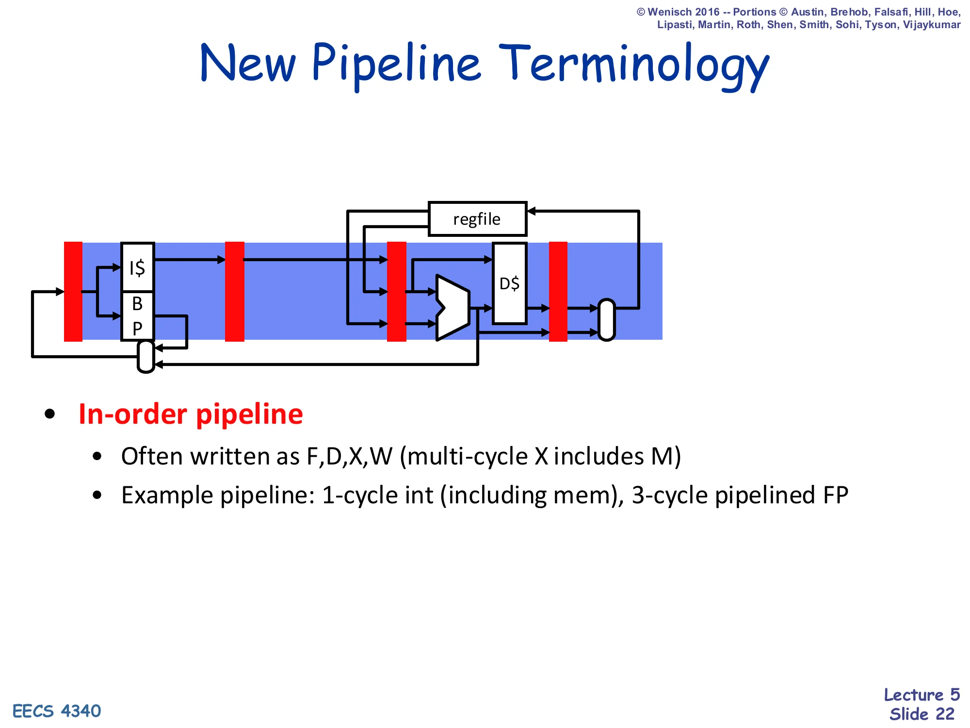
New Pipeline Terminology

In-order pipeline
- Often written as F, D, X, W (multi-cycle X includes M)
- Example pipeline: 1-cycle int (including mem), 3-cycle pipelined FP

(Diagram: in-order pipeline with I $+ BP feeding F → D → X (ALU/D$ ) → W, with feedback from W back to regfile.)

From here on, the lecture compresses the canonical 5-stage pipeline into four labels: F (fetch), D (decode), X (execute, possibly multi-cycle and including memory), and W (writeback). The in-order picture has one register (latch) per stage: each cycle exactly one instruction occupies each stage and a stall in any stage back-pressures every younger stage. The example processor used throughout the rest of the lecture has a 1-cycle integer execute (which subsumes memory), and a 3-cycle pipelined FP unit; this is the configuration used in all the cycle-by-cycle examples that follow. This four-letter naming will be repeated in scoreboard and Tomasulo with the addition of S (issue) between D and X.

New Pipeline Diagram (alternative)

Show slide text

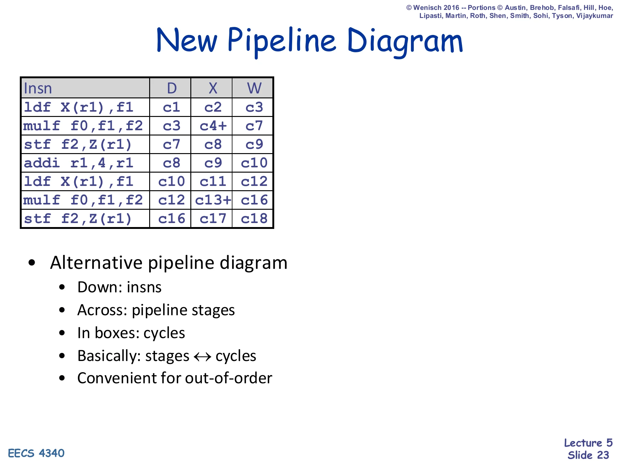
New Pipeline Diagram

Insn	D	X	W
`ldf X(r1),f1`	c1	c2	c3
`mulf f0,f1,f2`	c3	c4+	c7
`stf f2,Z(r1)`	c7	c8	c9
`addi r1,4,r1`	c8	c9	c10
`ldf X(r1),f1`	c10	c11	c12
`mulf f0,f1,f2`	c12	c13+	c16
`stf f2,Z(r1)`	c16	c17	c18

Alternative pipeline diagram
- Down: insns; Across: pipeline stages; In boxes: cycles
- Basically: stages ↔ cycles
- Convenient for out-of-order

This is the cycle-table notation that all the scoreboard examples use. Each row is one instruction, each column is one pipeline stage, and the entry in each box is the cycle in which that instruction occupied that stage. “c4+” denotes a multi-cycle execute that started in cycle 4 (the multi-cycle FP mulf takes c4–c6 and writes back in c7). The notation generalizes well to out-of-order execution because a row’s stages are no longer required to be contiguous in time: an instruction can sit in D for many cycles waiting to issue, then run through X and W normally. The two-iteration example here will reappear repeatedly: it is contrasted later against the scoreboard schedule of the same code to show what dynamic scheduling buys you.

The Problem With In-Order Pipelines (II)

Show slide text

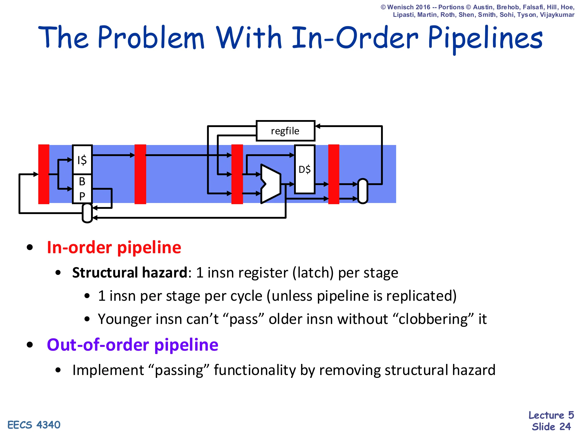
The Problem With In-Order Pipelines

In-order pipeline
- Structural hazard: 1 insn register (latch) per stage
  - 1 insn per stage per cycle (unless pipeline is replicated)
  - Younger insn can’t “pass” older insn without “clobbering” it
Out-of-order pipeline
- Implement “passing” functionality by removing structural hazard

The fundamental obstacle to letting a younger instruction skip past an older stalled one is a structural hazard: the in-order pipeline only has one latch in each stage, so if you let the younger instruction into D you would overwrite the older instruction sitting there. The fix is conceptual but also literal: replace that single decode latch with a pool of decode-stage storage (the instruction buffer), so the older stalled instruction has a place to wait while younger instructions stream past. The next slides build that pool — the instruction buffer — and then add the bookkeeping the scheduler needs to keep track of which buffered instruction is ready to run.

Instruction Buffer

Show slide text

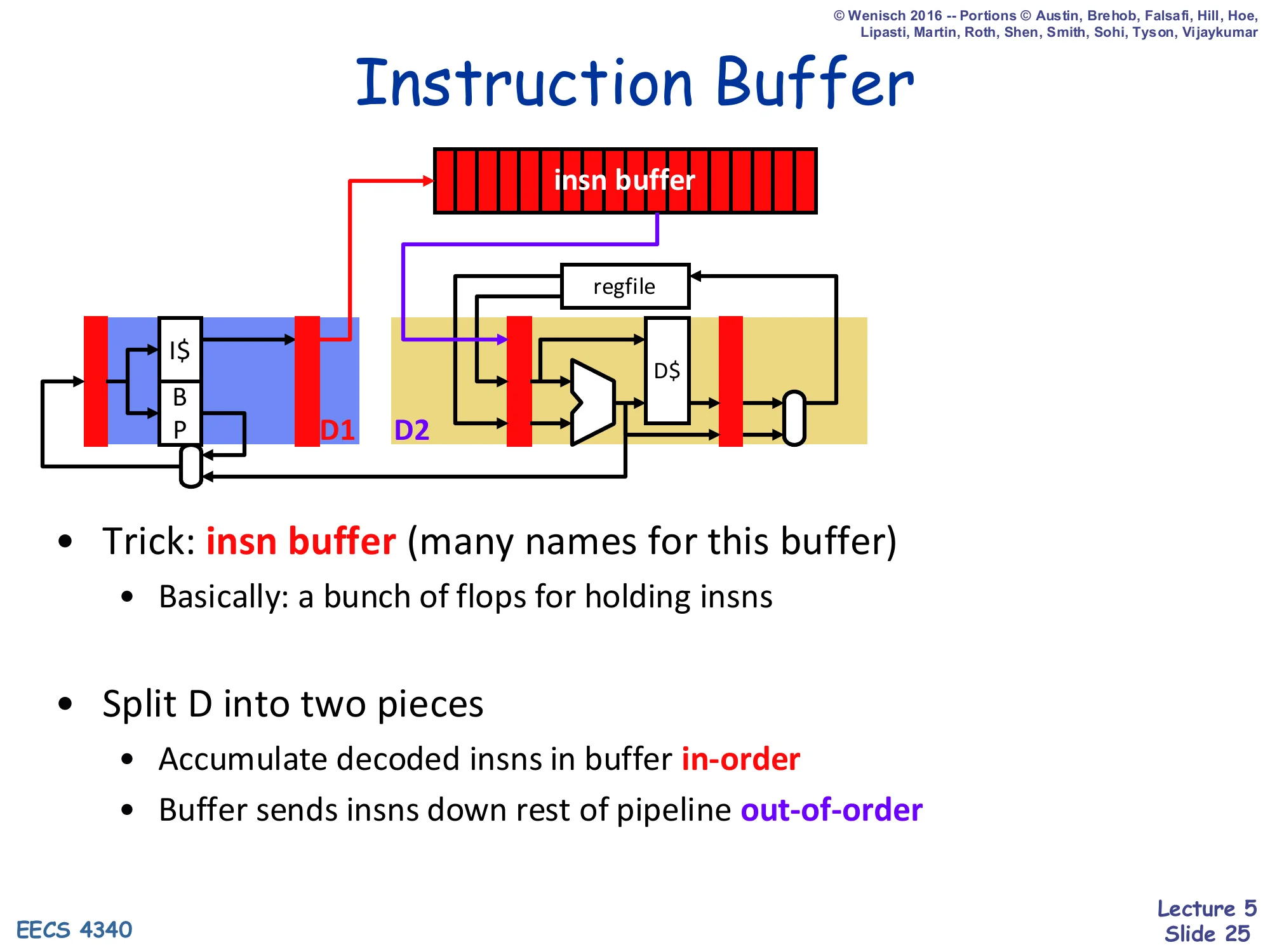
Instruction Buffer

Trick: insn buffer (many names for this buffer)
- Basically: a bunch of flops for holding insns
Split D into two pieces
- Accumulate decoded insns in buffer in-order
- Buffer sends insns down rest of pipeline out-of-order

The insn buffer is the storage that breaks the structural hazard of slide 24. Decode is split into two phases: D1 fills the buffer in program order (so renaming/dispatch state stays sequential), and D2 picks instructions out of the buffer in whatever order the hardware deems ready, dispatching them down the rest of the pipeline. This split is the heart of every dynamic-scheduling design: the insn buffer shows up under many names — instruction window, instruction scheduler, reservation stations (Tomasulo), or the integrated FUST entries (scoreboard). The differences between scoreboard, Tomasulo, P6, and R10K are largely about what this buffer stores per entry and how it tracks readiness.

Dispatch and Issue

Show slide text

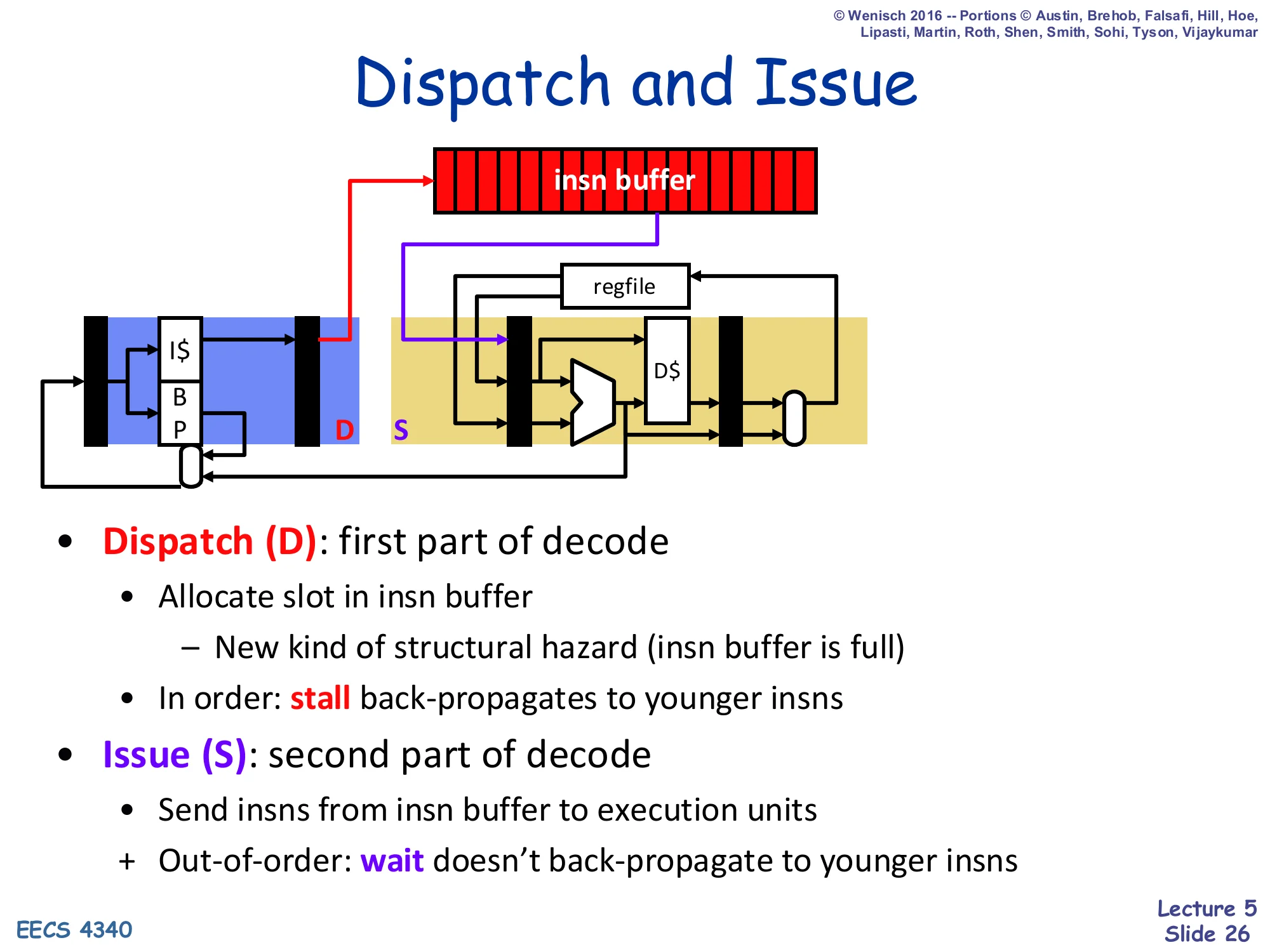
Dispatch and Issue

Dispatch (D): first part of decode
- Allocate slot in insn buffer
  - New kind of structural hazard (insn buffer is full)
- In order: stall back-propagates to younger insns
Issue (S): second part of decode
- Send insns from insn buffer to execution units
- $+$ Out-of-order: wait doesn’t back-propagate to younger insns

This slide nails down the two new pipeline stages. Dispatch (D) is in-order: each cycle the dispatch logic takes the next decoded instruction and tries to allocate it a slot in the insn buffer (and a free FU entry, in scoreboard). If the buffer is full or a needed FU is busy, dispatch must stall, and that stall back-propagates to all younger instructions because they cannot get past the in-order dispatch pipe. Issue (S) is out-of-order: each cycle the issue logic looks across all the buffer entries, picks any whose operands are ready, and fires them into the FU. Crucially, when an entry has to wait for its operands, that wait does not delay any younger entry — that is the entire point of dynamic scheduling. The new pipeline structure is therefore F, D, S, X, W, and these five letters appear in every scoreboard cycle-table from now on.

Dispatch and Issue with Floating-Point

Show slide text

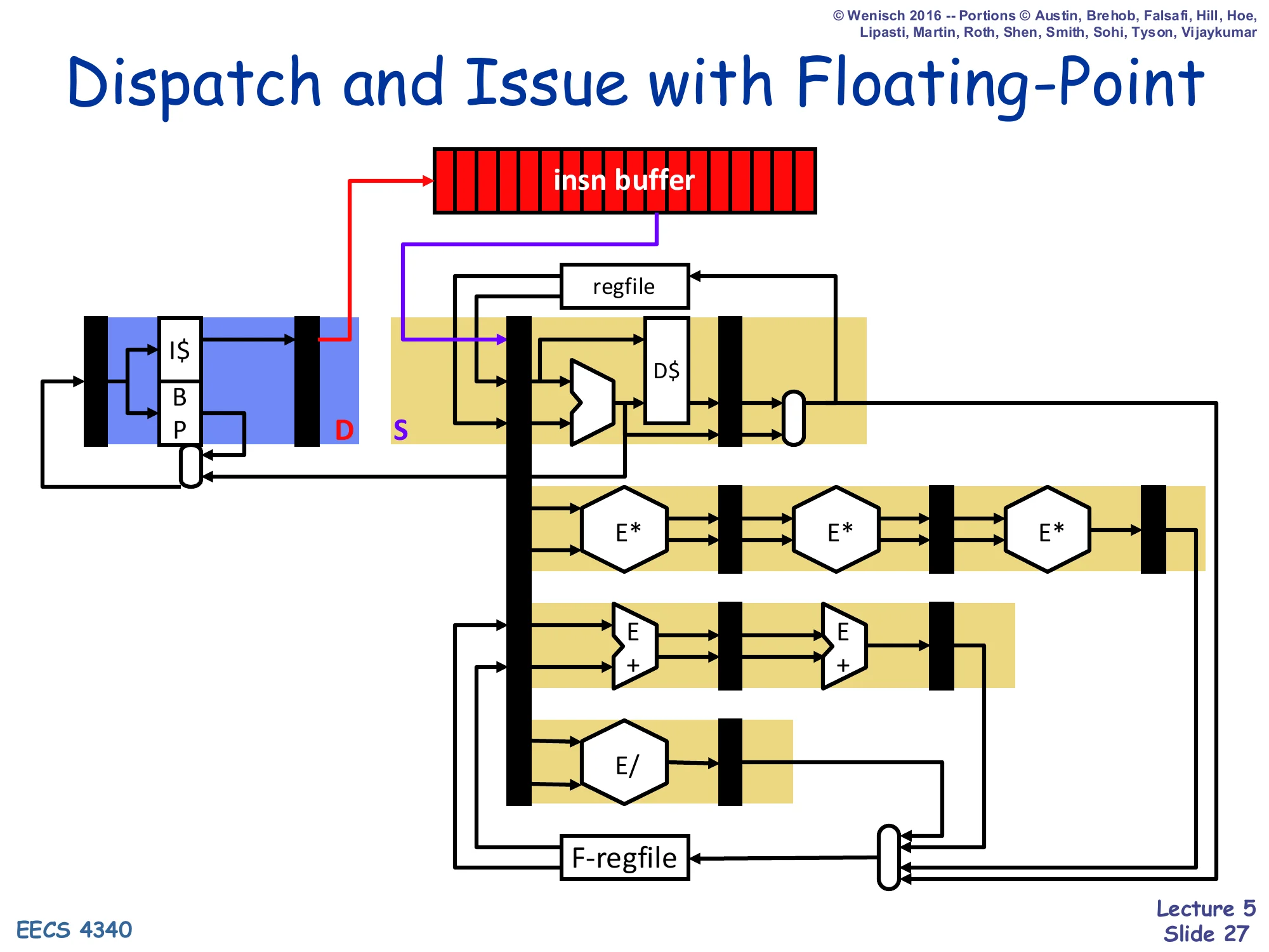
Dispatch and Issue with Floating-Point

(Diagram: insn buffer feeds an issue port that sprays into multiple parallel functional units — integer/D-cache, a 3-stage E* (FP multiply) pipeline, a 2-stage E+ (FP add) pipeline, and a non-pipelined E/ (FP divide). Each FU has its own writeback latch into the F-regfile.)

Adding floating point makes the value of the instruction buffer obvious: different FP operations have wildly different latencies (3-stage pipelined multiply, 2-stage pipelined add, non-pipelined divide), so a single in-order pipeline either has to be padded out to the worst case or has to forbid issuing FP behind any other FP. The buffer-plus-multiple-FU diagram lets the issue logic send each instruction to its appropriate unit and hold the rest in the buffer until ready. The integer side and the FP side share one buffer but have separate execute pipelines and separate writeback ports back into their respective register files. This is exactly the style of organization used in the simple scoreboard introduced on slide 29: 5 functional units (1 ALU, 1 LD, 1 ST, 2 FP) each with its own status entry.

Dynamic Scheduling Algorithms

Show slide text

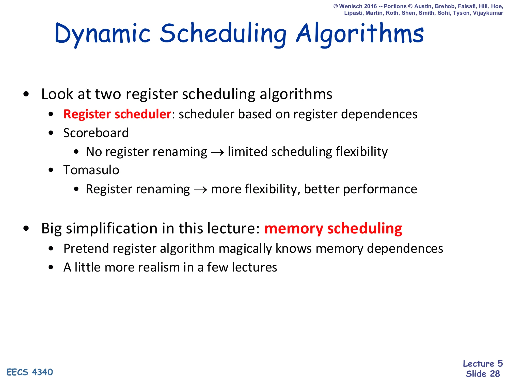
Dynamic Scheduling Algorithms

Look at two register scheduling algorithms
- Register scheduler: scheduler based on register dependences
- Scoreboard
  - No register renaming → limited scheduling flexibility
- Tomasulo
  - Register renaming → more flexibility, better performance
Big simplification in this lecture: memory scheduling
- Pretend register algorithm magically knows memory dependences
- A little more realism in a few lectures

The lecture restricts attention to register scheduling. Scoreboarding is centralized and does not rename, so it inherits the full WAR/WAW pain. Tomasulo adds renaming and gets more reordering freedom. Memory scheduling is much harder because addresses are computed in the X stage, not at decode/rename: the hardware does not know whether a load and an older store touch the same address until the addresses arrive. The lecture explicitly hand-waves this: it pretends that the moment a load or store appears, the hardware magically knows which prior memory operations it conflicts with. Real implementations use store-buffer-with-forwarding plus speculative load issue plus replay-on-conflict; that is the memory disambiguation story for L09.

Scheduling Algorithm I: Scoreboard

Show slide text

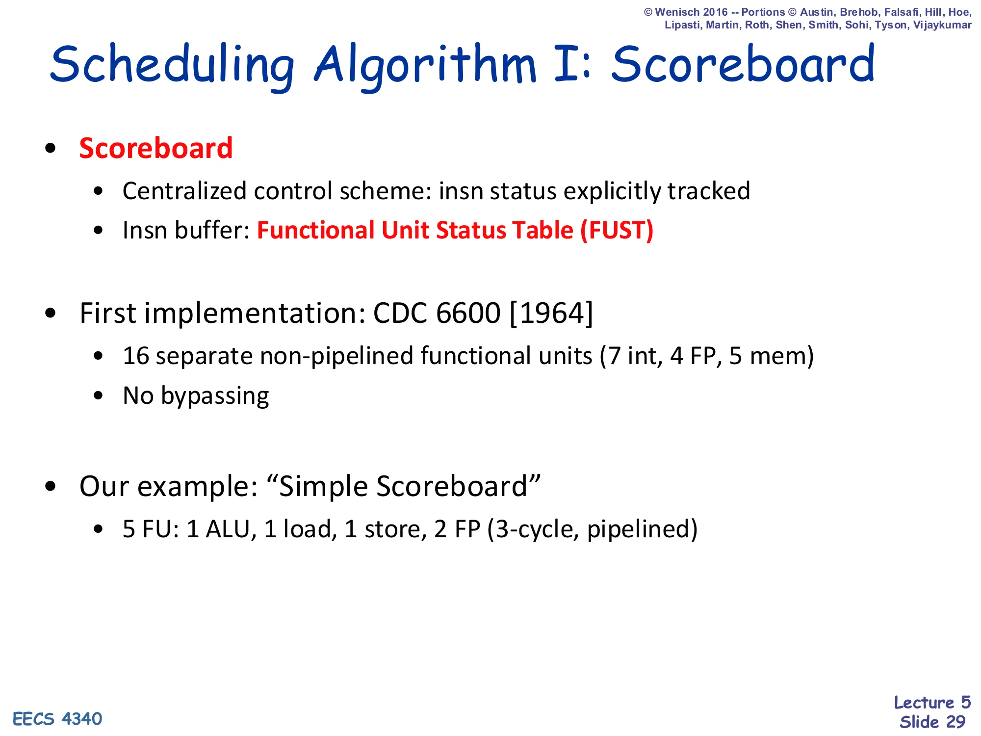
Scheduling Algorithm I: Scoreboard

Scoreboard
- Centralized control scheme: insn status explicitly tracked
- Insn buffer: Functional Unit Status Table (FUST)
First implementation: CDC 6600 [1964]
- 16 separate non-pipelined functional units (7 int, 4 FP, 5 mem)
- No bypassing
Our example: “Simple Scoreboard”
- 5 FU: 1 ALU, 1 load, 1 store, 2 FP (3-cycle, pipelined)

Scoreboarding is a centralized hardware-tracking scheme: a single block of state — the scoreboard — records the status of every in-flight instruction and every architectural register. The insn buffer in this design is not a separate flat array but is folded into the per-FU “Functional Unit Status Table” (FUST), which holds one waiting instruction per FU. The CDC 6600 (1964) was the first real machine to use this approach; it had 16 functional units and explicitly no bypass network — the scoreboard handled all scheduling instead. The lecture’s running example is a smaller “Simple Scoreboard” with 5 FUs (1 ALU, 1 load, 1 store, and 2 pipelined 3-cycle FP units). Every cycle-by-cycle example for the rest of the lecture uses this configuration.

Scoreboard Data Structures

Show slide text

Scoreboard Data Structures

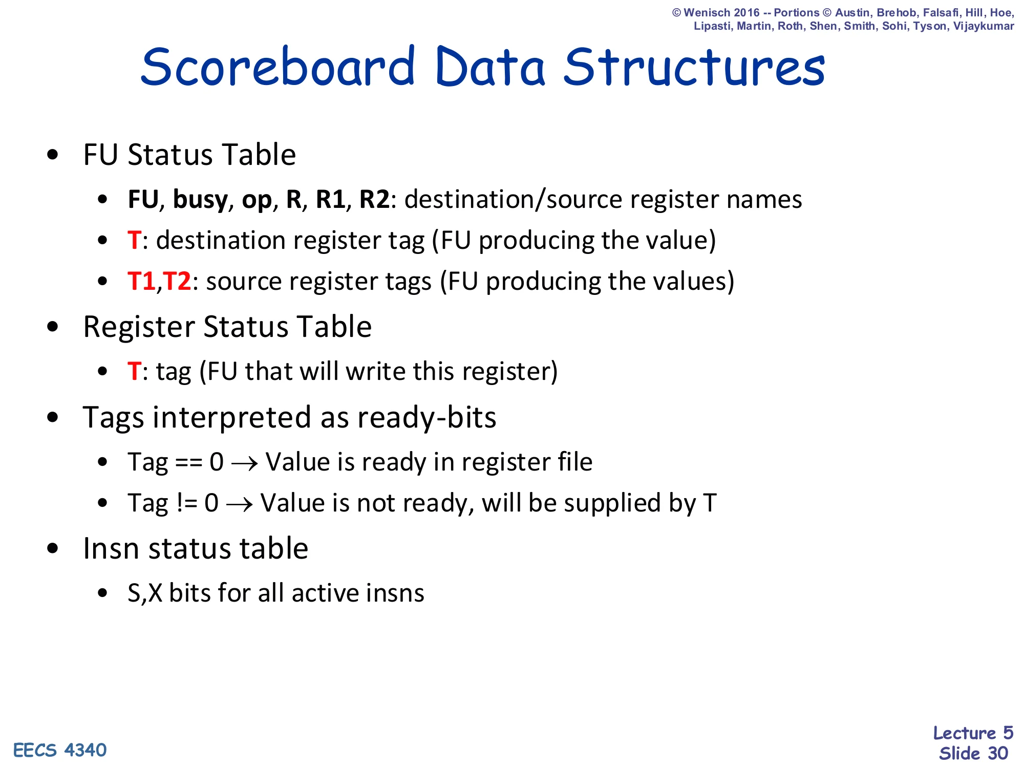
FU Status Table
- FU, busy, op, R, R1, R2: destination/source register names
- T: destination register tag (FU producing the value)
- T1, T2: source register tags (FU producing the values)
Register Status Table
- T: tag (FU that will write this register)
Tags interpreted as ready-bits
- Tag == 0 → Value is ready in register file
- Tag != 0 → Value is not ready, will be supplied by T
Insn status table
- S, X bits for all active insns

The scoreboard’s three tables are the key data structures. FU Status Table: one row per functional unit, holding the destination and source register names (R, R1, R2), the destination tag T (which FU is producing the result), and source tags T1, T2 (which FUs are producing each operand). Register Status Table: one row per architectural register, holding the tag T = the FU that will eventually write that register; T = 0 means the value is currently in the regfile and ready. Insn Status Table: per-instruction S/X bits showing where each in-flight instruction is in the pipeline. The convention “tag == 0 → ready” is critical: an issuing instruction copies T1 and T2 from the Register Status Table at dispatch, then sits in its FU entry until both T1 == 0 and T2 == 0, at which point it can read the regfile and issue.

Simple Scoreboard Data Structures

Show slide text

Simple Scoreboard Data Structures

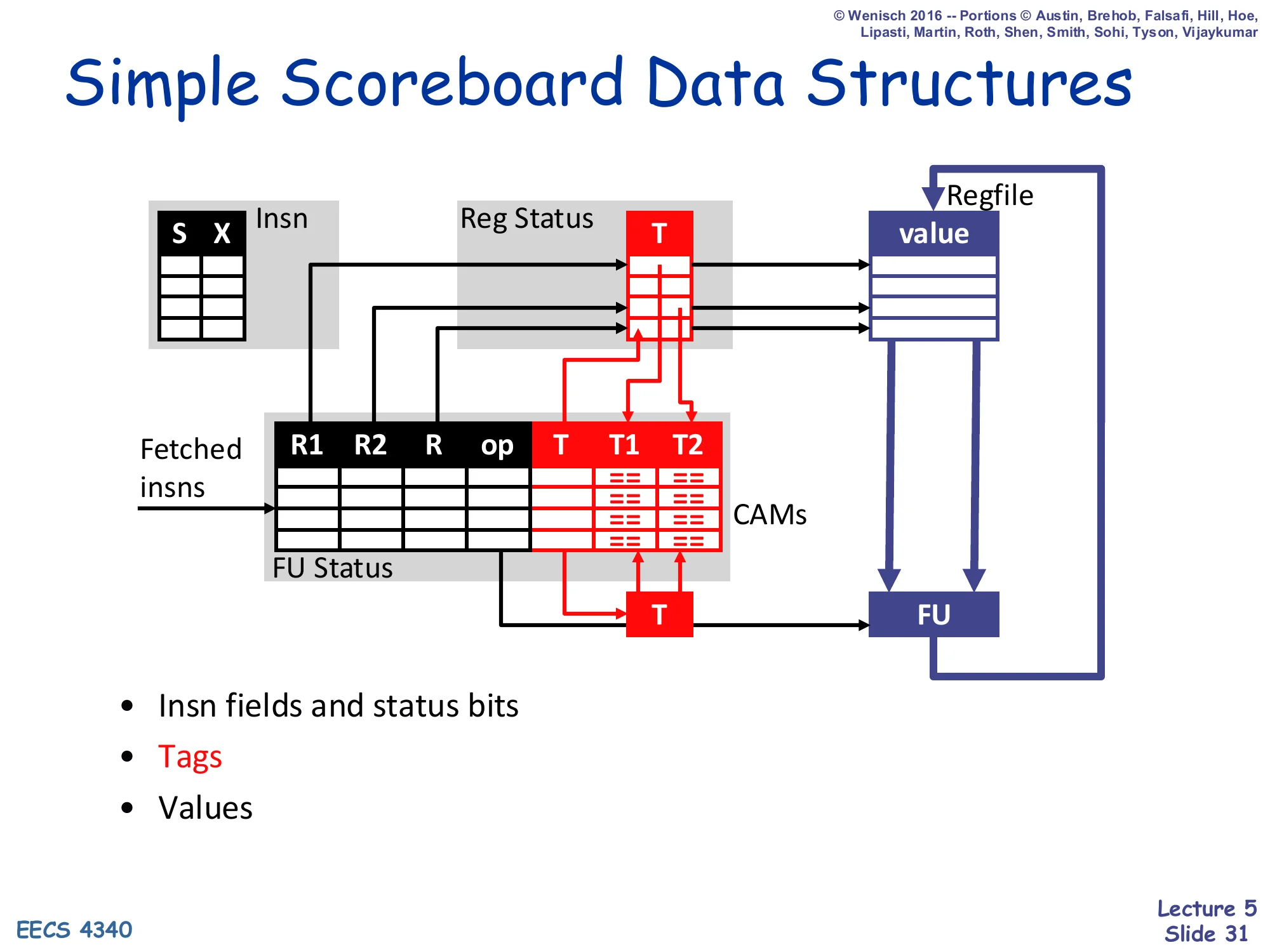
Diagram showing four cooperating tables and the regfile:

Insn (S, X) — per-insn status bits
Reg Status (T) — per-regfile-register tag pointing to the FU that will write it
FU Status (R1, R2, R, op, T, T1, T2) — per-FU instruction info plus tags
Regfile (value) — actual data
T compares (CAMs) on T1, T2 inputs to detect when a writing FU’s tag matches a waiting FU’s source tag
Insn fields and status bits
Tags
Values

This diagram zooms in on the tag-matching machinery. The “T” column on the right of FU Status (the destination tag) is broadcast back to the T1 and T2 CAMs of every FU entry; whenever a writing FU’s tag matches a waiting entry’s source tag, that source tag is cleared (”== 0”), making the operand ready. The Reg Status table forwards each register’s currently-pending tag T into the FU Status when an instruction dispatches, so that the dispatching instruction inherits the correct producer tag rather than silently reading a stale value. The CAMs (Content Addressable Memories) are the implementation cost: every cycle, the destination tag of any writing FU must be compared against every source tag in every FU entry. This wide associative compare is exactly why scoreboards stay small and why renaming-based schemes (Tomasulo) eventually win.

Scoreboard Pipeline

Show slide text

Scoreboard Pipeline

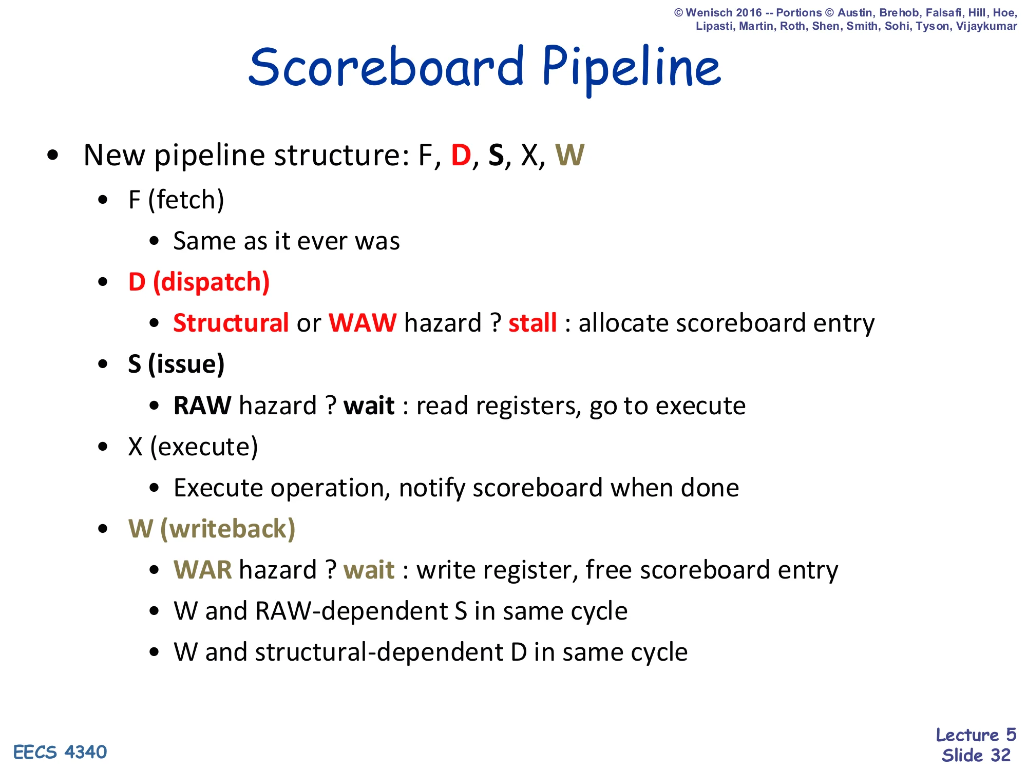
New pipeline structure: F, D, S, X, W
- F (fetch) — same as it ever was
- D (dispatch)
  - Structural or WAW hazard? stall : allocate scoreboard entry
- S (issue)
  - RAW hazard? wait : read registers, go to execute
- X (execute) — execute operation, notify scoreboard when done
- W (writeback)
  - WAR hazard? wait : write register, free scoreboard entry
  - W and RAW-dependent S in same cycle
  - W and structural-dependent D in same cycle

This single slide defines the scoreboard’s full life-cycle rules — and, equivalently, where it pays for each kind of hazard. D is the in-order checkpoint: it stalls on a structural hazard (FU busy or scoreboard entry unavailable) or on a WAW hazard (Reg Status[R] non-empty means an older in-flight instruction is going to write the same register). S waits on a RAW hazard until both source tags have been cleared. X does the actual work and signals back. W waits on a WAR hazard — it cannot overwrite the architectural register until any older instruction that reads that register has already issued from S. The two “in same cycle” footnotes are the bypass concessions that prevent the dispatch and issue stages from being pessimistic by one cycle. Every cycle-by-cycle scoreboard example after this slide is just an application of these rules.

Scoreboard Dispatch (D)

Show slide text

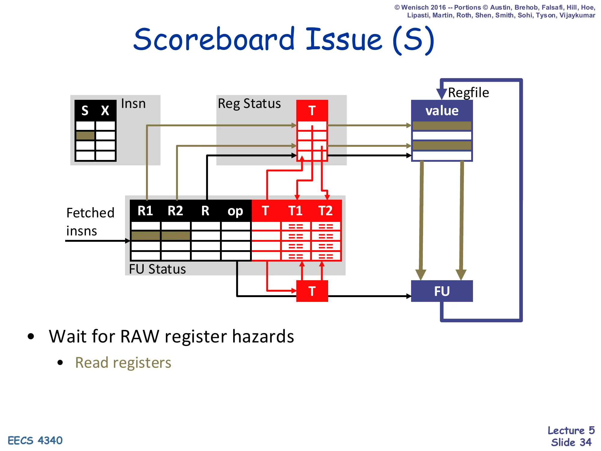
Scoreboard Dispatch (D)

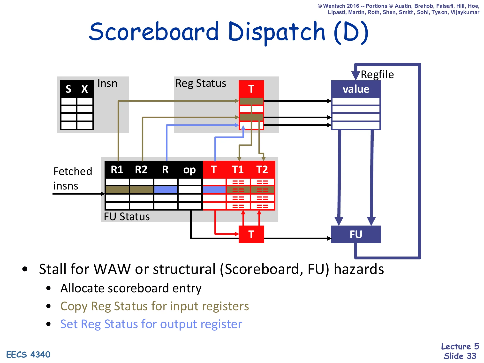
(Diagram: at dispatch, a fetched insn lands in an FU Status row. The insn’s source tags T1, T2 are copied from the Reg Status table for R1 and R2 inputs. The insn’s destination tag T is set in Reg Status for R, marking that this FU will eventually write R.)

Stall for WAW or structural (Scoreboard, FU) hazards
Allocate scoreboard entry
Copy Reg Status for input registers
Set Reg Status for output register

Dispatch is the only in-order transition. Three things happen simultaneously when a new instruction successfully dispatches: (1) an FU Status row is allocated for it (this is the structural hazard check — that FU must be free and the scoreboard must not have an existing writer for the same destination, the WAW check); (2) the current Reg Status[R1] and Reg Status[R2] tags are copied into FU Status T1, T2 — the dispatching instruction inherits whatever in-flight FU will eventually produce its operands; (3) Reg Status[R] is set to point to this FU, telling future dispatchers that any subsequent reader of R will need to wait on this FU’s tag. If any of those checks fails, the instruction blocks in D, and because D is in-order every younger instruction blocks behind it.

Scoreboard Issue (S)

Show slide text

Scoreboard Issue (S)

(Diagram: at issue, a waiting FU entry whose T1 and T2 tags are both clear reads its R1, R2 values from the regfile and ships them to the FU’s input latches.)

Wait for RAW register hazards
Read registers

Issue is the out-of-order step. Every cycle, the issue logic scans the FU Status table for any entry whose T1 and T2 tags are both 0 (i.e., both source operands are ready in the register file). At most one such ready entry is selected per FU and read out; its R1 and R2 register names are sent to the regfile, the values come back, and the FU begins execution. Until both source tags have been cleared by some prior writeback, the entry simply waits — but waiting in S, unlike stalling in D, does not block any younger instruction in some other FU. This is exactly the asymmetry between dispatch and issue introduced on slide 26: stall propagates back to younger insns, wait does not. The only register hazard checked at issue is the RAW hazard.

Issue Policy and Issue Logic

Show slide text

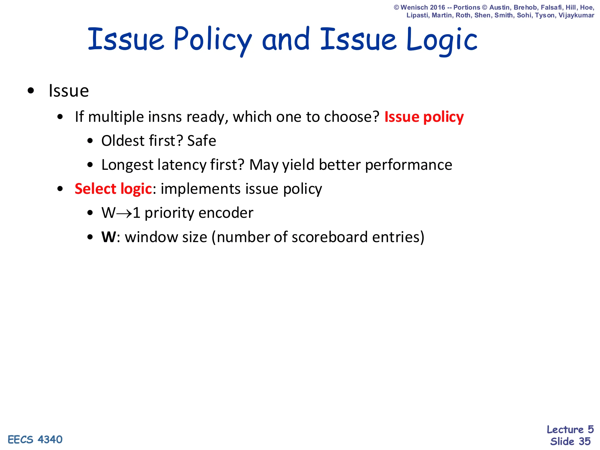
Issue Policy and Issue Logic

Issue
- If multiple insns ready, which one to choose? Issue policy
  - Oldest first? Safe
  - Longest latency first? May yield better performance
- Select logic: implements issue policy
  - W → 1 priority encoder
  - W: window size (number of scoreboard entries)

When several FU entries become ready simultaneously, the hardware must pick one. The textbook “oldest first” rule (largest sequential age) is conservative and safe: it never starves an older instruction and tends to preserve precise-state intuitions. “Longest latency first” can win in practice because firing a long-latency op (e.g., FP divide) earlier overlaps more of its latency with subsequent work. The implementation is a select logic circuit — basically a priority encoder over the W ready-bits in the window. Window size W is a fundamental performance knob: a wider window finds more ILP but the priority encoder grows roughly $O(W)$ in fan-in and area. This generic discussion applies to Tomasulo and modern OoO machines as well — only the data structures change.

Scoreboard Execute (X)

Show slide text

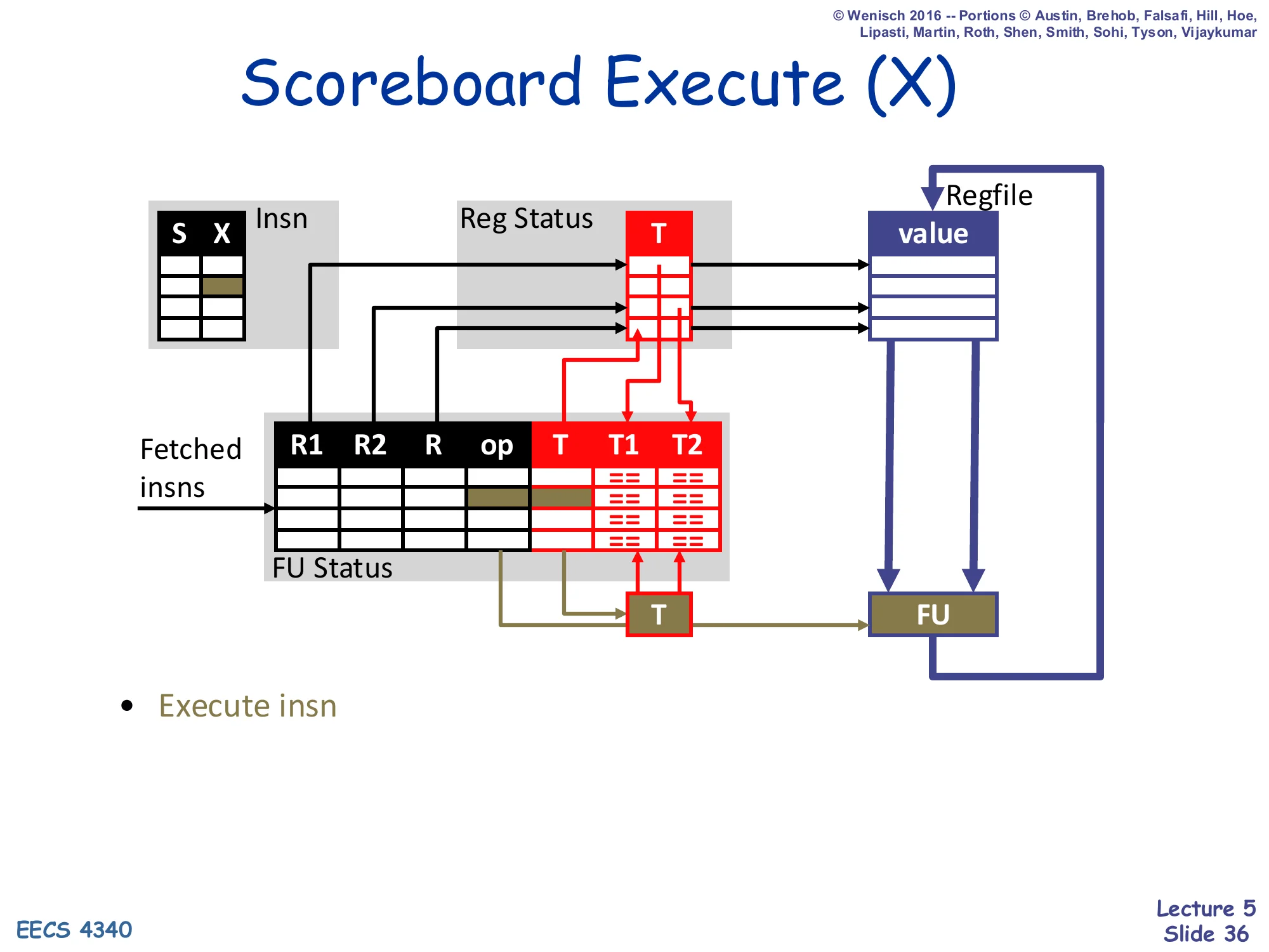
Scoreboard Execute (X)

(Diagram: the FU runs through its execute stages with the values read at issue. The Insn Status X bit is set; for a multi-cycle FU like the 3-cycle FP multiplier, the X stage spans multiple cycles.)

Execute insn

Execute is the simplest stage in the scoreboard’s life cycle. Once the operands have been read from the regfile in S, the values flow into the FU and the FU does its work — this can be one cycle (ALU, simple integer) or multiple cycles (3-cycle pipelined FP multiply). The FU is now the only consumer of the stale architectural register values it read, which is what makes the WAR check at writeback necessary: a younger writer cannot overwrite the architectural register until this FU’s instruction has finished reading it and entered execute. There is no scheduling decision in X — the only thing that happens here is the operation completes and the writeback stage requests Reg Status.

Scoreboard Writeback (W)

Show slide text

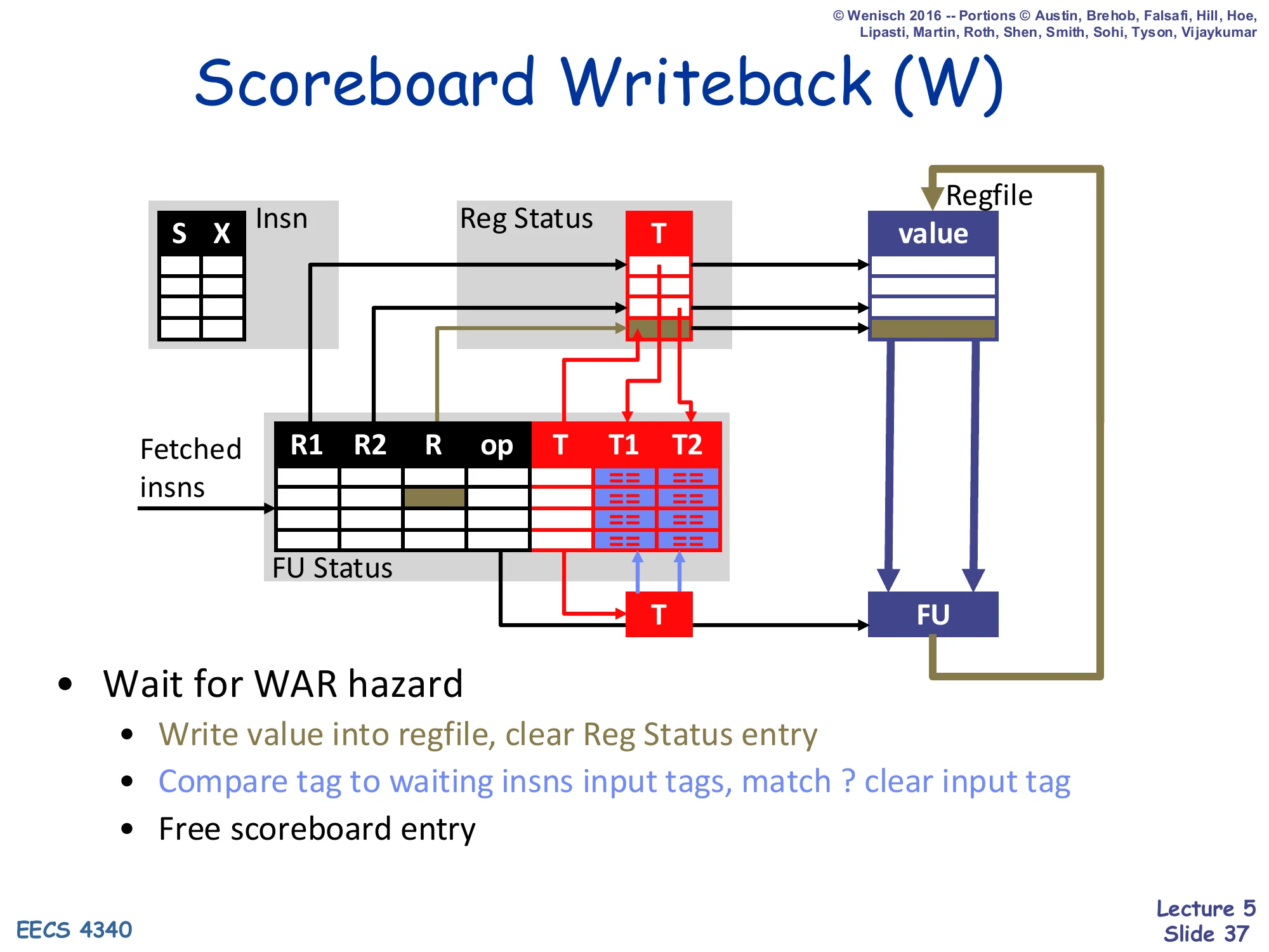
Scoreboard Writeback (W)

(Diagram: at writeback, the FU’s destination tag T is broadcast on a tag bus. Every waiting FU entry’s T1 and T2 CAM cells compare against the broadcast T; matches clear those input tags. The result value is written into the regfile, and Reg Status[R] is cleared.)

Wait for WAR hazard
Write value into regfile, clear Reg Status entry
Compare tag to waiting insns input tags, match? clear input tag
Free scoreboard entry

Writeback does three things at once. First, it must wait for any in-flight older reader of the destination architectural register R — that is the WAR check, implemented by scanning the FU Status table for any entry whose R1 or R2 still names R but whose corresponding T1/T2 is 0 (meaning that older instruction has read R from the regfile and is sitting in execute, but its WAR sister has not yet been resolved). Second, it broadcasts the writing FU’s tag T on the tag bus; every CAM cell across the FU Status T1, T2 columns compares — matches clear those source tags, which is what makes downstream RAW-dependent instructions ready. Third, the result value is written into the regfile, Reg Status[R] is cleared (becomes “0 = ready in regfile”), and the FU Status row is freed for reallocation.

Scoreboard Data Structures (initial)

Show slide text

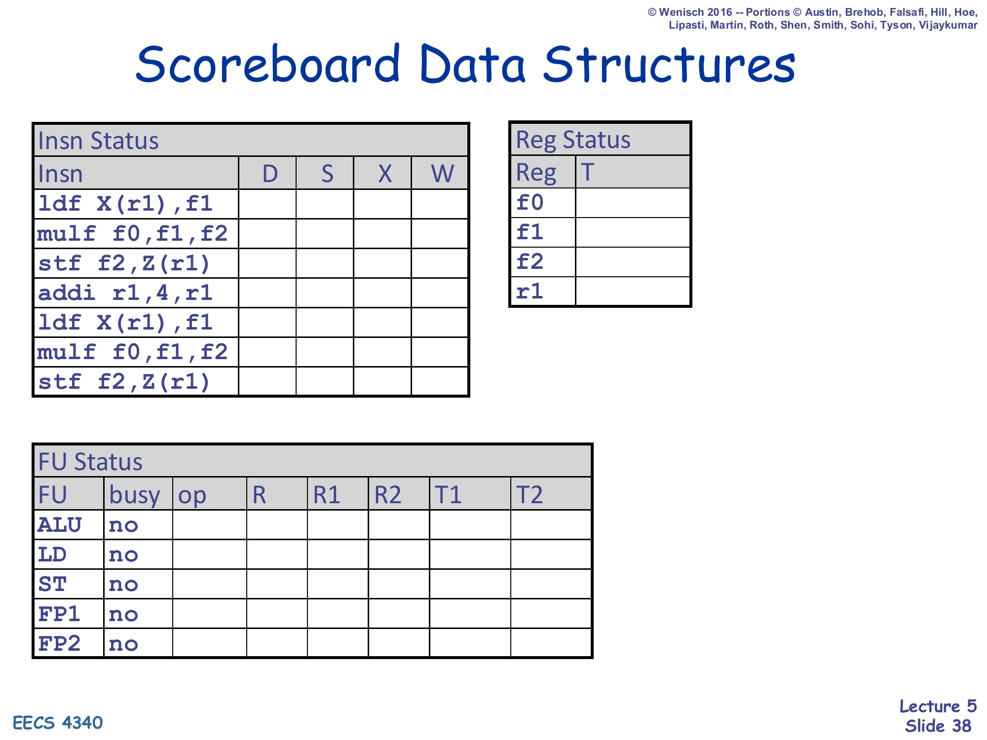
Scoreboard Data Structures

Insn Status (initial — all blank)

Insn	D	S	X	W
`ldf X(r1),f1`
`mulf f0,f1,f2`
`stf f2,Z(r1)`
`addi r1,4,r1`
`ldf X(r1),f1`
`mulf f0,f1,f2`
`stf f2,Z(r1)`

Reg Status (initial — empty)

Reg	T
f0
f1
f2
r1

FU Status (initial — busy = no for all)

FU	busy	op	R	R1	R2	T1	T2
ALU	no
LD	no
ST	no
FP1	no
FP2	no

This is the starting state for the running scoreboard example: seven instructions to execute (two iterations of the loop ldf; mulf; stf; addi), three tracking tables, all empty. The instruction sequence is the same one used in the in-order example on slide 23, so the eventual schedule can be compared one-to-one. The 5 FUs match the simple-scoreboard configuration: 1 ALU, 1 LD, 1 ST, 2 FP. The Reg Status table tracks four architectural registers (f0, f1, f2, r1) — only those that appear as destinations or sources in the snippet. The Insn Status table will be filled in cycle-by-cycle in the slides that follow, with each instruction proceeding through D, S, X, and W as the rules of slide 32 allow.

Scoreboard: Cycle 1

Show slide text

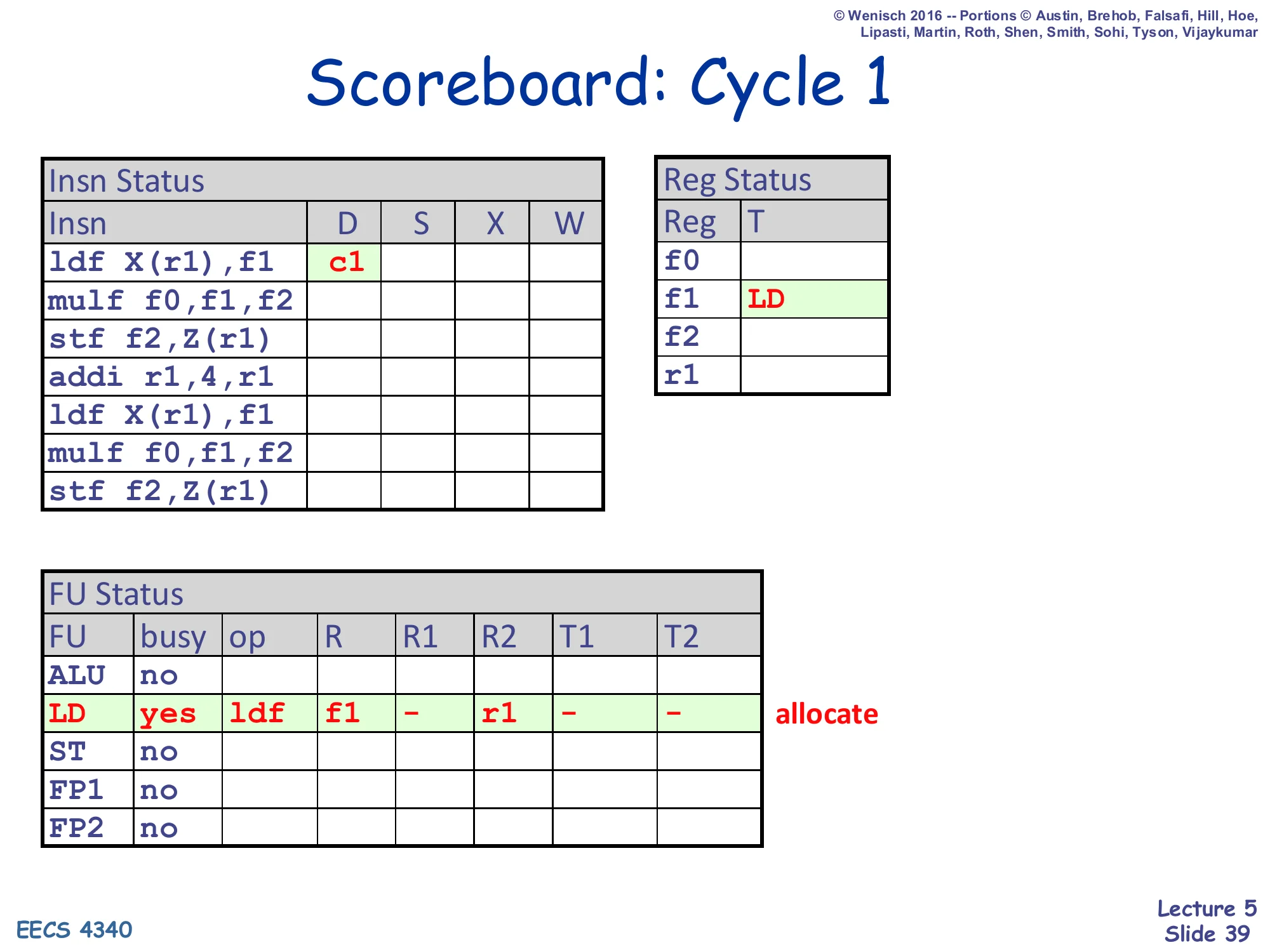
Scoreboard: Cycle 1

Insn Status — ldf X(r1),f1: D = c1

Reg Status — f1: T = LD

FU Status — LD row allocated: busy=yes, op=ldf, R=f1, R1=–, R2=r1, T1=–, T2=–

Cycle 1: the first ldf X(r1),f1 dispatches. The LD FU is free and no one is currently writing f1 (no structural or WAW hazard), so the dispatch succeeds. The LD row is allocated with op=ldf and the source register r1 (T2 inherits Reg Status[r1] which is empty, so T2 = 0/–). The destination is f1 with no source operand on R1 (immediate offset). Reg Status[f1] is now set to LD, telling any future reader of f1 that it must wait for the LD unit’s tag. The Insn Status row records D=c1; S can happen as early as next cycle once the issue logic sees the entry.

Scoreboard: Cycle 2

Show slide text

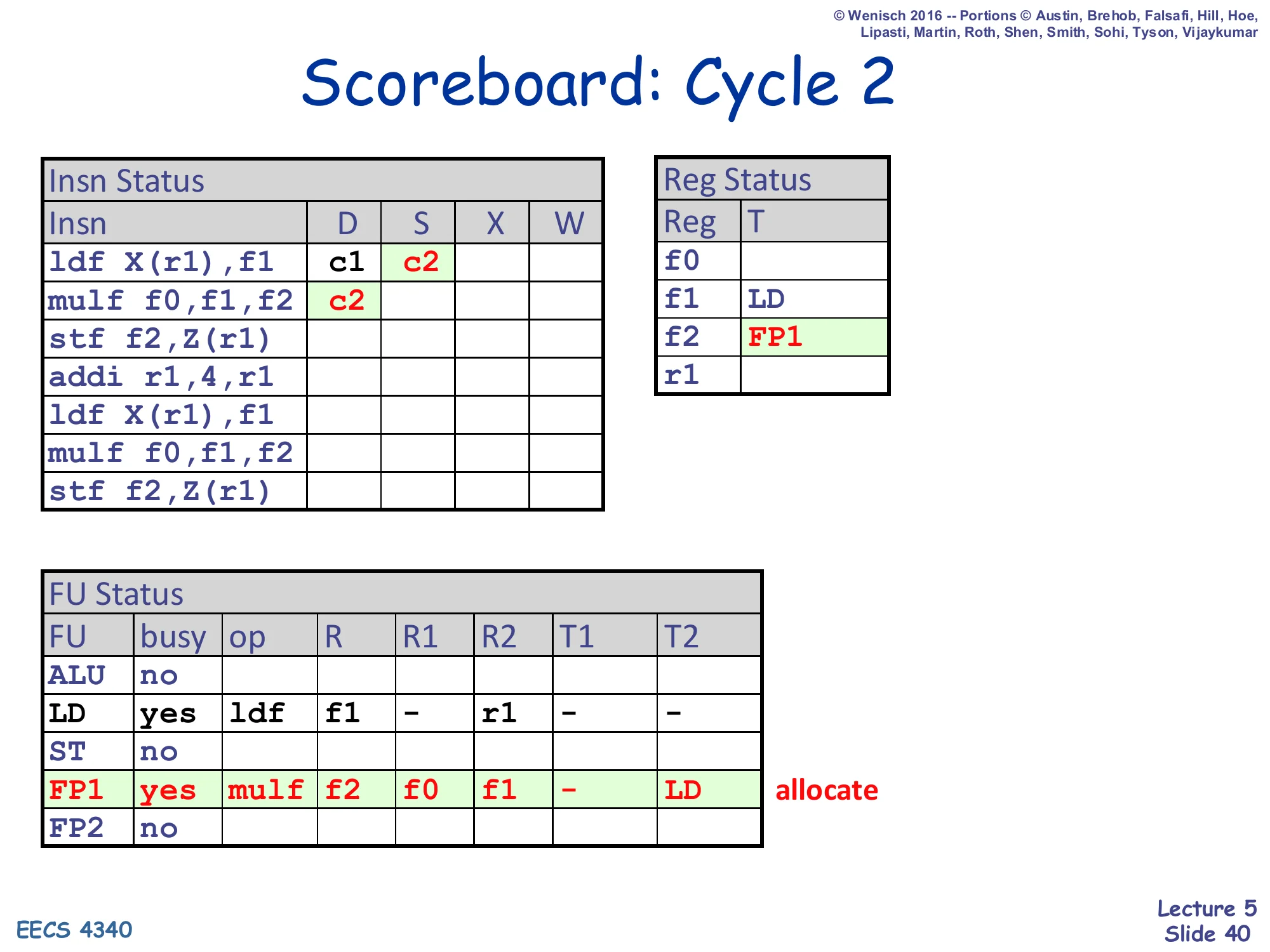
Scoreboard: Cycle 2

Insn Status — ldf X(r1),f1: D=c1, S=c2; mulf f0,f1,f2: D=c2

Reg Status — f1: LD; f2: FP1

FU Status — LD row holds ldf (R=f1, R2=r1); FP1 row newly allocated for mulf: op=mulf, R=f2, R1=f0, R2=f1, T1=–, T2=LD

Cycle 2: two things happen at once. The first ldf issues (S = c2) — both source tags are clear (r1 is in the regfile, no immediate-side tag), so it reads its operands and proceeds toward execute. The second instruction mulf f0,f1,f2 dispatches into the FP1 unit. Crucially, when mulf dispatches it copies the current Reg Status: f0 is empty (T1 = –), f1 is LD (so T2 = LD — mulf is now waiting on the LD unit’s tag). Reg Status[f2] is set to FP1 to reflect that FP1 will eventually write f2. There is no RAW or WAW issue at dispatch — RAW will be checked later, in S. The mulf cannot issue this cycle because T2 = LD (still pending).

Scoreboard: Cycle 3

Show slide text

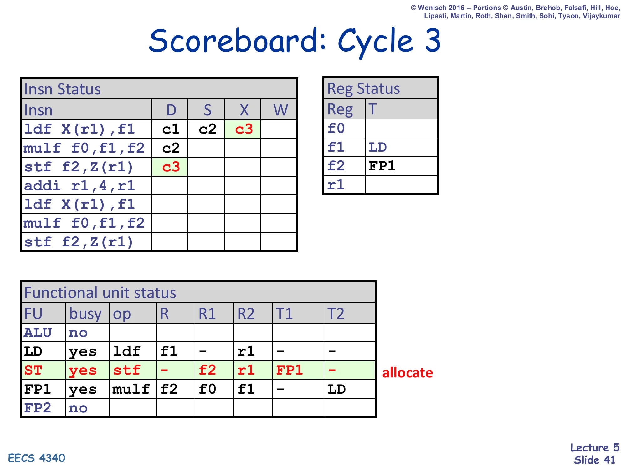
Scoreboard: Cycle 3

Insn Status — ldf: D=c1, S=c2, X=c3; mulf: D=c2; stf f2,Z(r1): D=c3

Reg Status — f1: LD; f2: FP1

FU Status — ldf in LD; mulf in FP1 (T2=LD); ST row newly allocated for stf: op=stf, R=–, R1=f2, R2=r1, T1=FP1, T2=–

Cycle 3: ldf reaches execute (X = c3) — it is a 1-cycle integer-style memory op so it will writeback next cycle. The mulf is still stuck in S because Reg Status said its f1 source comes from LD, and LD has not yet broadcast its writeback tag. The third instruction stf f2,Z(r1) dispatches into the ST FU. Stf reads f2 (T1 inherits FP1 — mulf is going to produce f2) and r1 (T2 = – because Reg Status[r1] is still empty). It has no destination register R, so Reg Status is not modified. So at cycle 3 we already have three instructions in flight in three different FUs (LD, FP1, ST), all at different stages — that is dynamic scheduling at work.

Scoreboard: Cycle 4

Show slide text

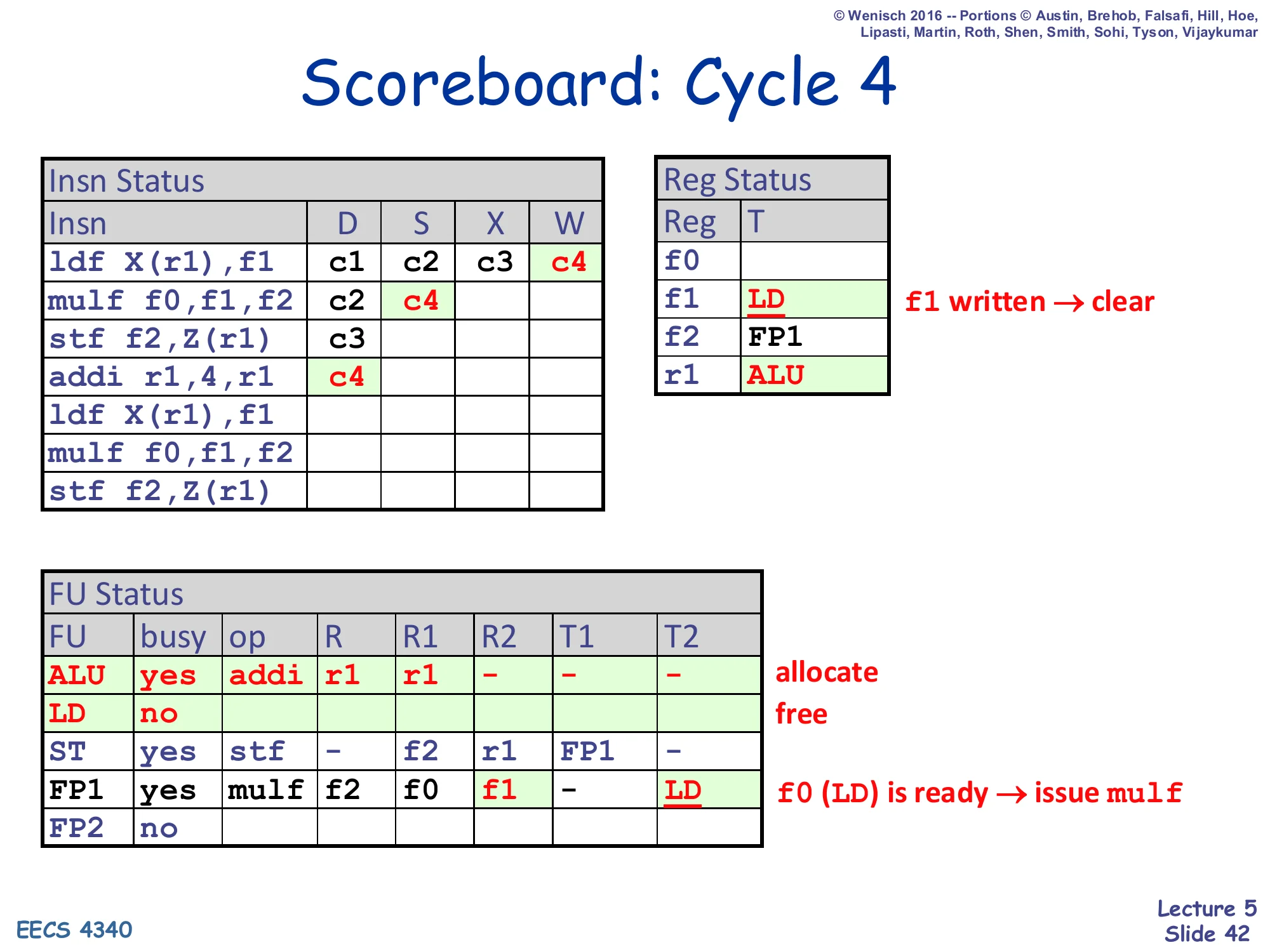
Scoreboard: Cycle 4

Insn Status — ldf: D=c1, S=c2, X=c3, W=c4; mulf: D=c2, S=c4; stf: D=c3; addi r1,4,r1: D=c4

Reg Status — f1: LD (cleared, f1 written → ready); f2: FP1; r1: ALU (newly set)

FU Status — ALU newly allocated for addi: op=addi, R=r1, R1=r1, T1=–; LD freed (busy=no); mulf’s T2 cleared (LD broadcast tag matched FP1.T2=LD, now both source tags are 0 → mulf can issue this cycle)

Cycle 4 is the busiest cycle yet — three concurrent activities. (1) ldf writes back: Reg Status[f1] is cleared and the LD FU is freed, and the LD’s destination tag is broadcast. The CAM in FP1’s T2 column matches, so FP1.T2 becomes 0. (2) Now that mulf has both source tags clear, it issues this cycle (S = c4) — “W and RAW-dependent S in same cycle” rule from slide 32 firing exactly. (3) The fourth instruction addi r1,4,r1 dispatches into the ALU; it writes r1 so Reg Status[r1] is set to ALU. Note carefully that mulf’s S happens in the same cycle as ldf’s W — without that bypass concession, mulf would have to wait an extra cycle. This is also the cycle the LD FU becomes free, allowing the second ldf to dispatch into it next cycle.

Scoreboard: Cycle 5

Show slide text

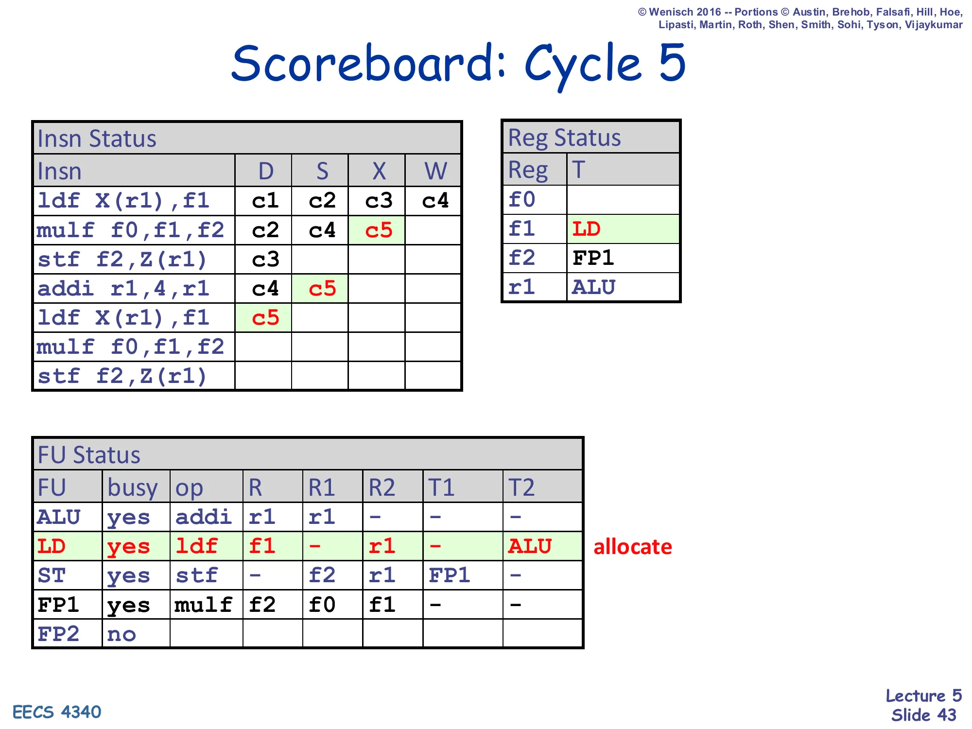
Scoreboard: Cycle 5

Insn Status — ldf₁: c1,c2,c3,c4; mulf₁: D=c2, S=c4, X=c5; stf₁: D=c3; addi: D=c4, S=c5; ldf₂ (second iteration): D=c5

Reg Status — f1: LD (re-set by ldf₂); f2: FP1; r1: ALU

FU Status — ALU: addi (R=r1, R1=r1, T1=–); LD newly allocated for ldf₂: R=f1, R2=r1, T2=ALU (because Reg Status[r1] = ALU, the addi will produce r1); ST: stf (T1=FP1); FP1: mulf executing

Cycle 5: addi issues from S into the ALU (its only source r1 is in the regfile), and the second-iteration ldf dispatches into the now-free LD FU. Look carefully at what the second ldf inherits: it reads r1, but Reg Status[r1] is currently ALU (because addi is going to produce the new r1), so ldf₂.T2 = ALU — ldf₂ has correctly recognized its RAW dependency on the addi’s r1 write without any explicit data forwarding. Reg Status[f1] is set to LD again (re-set, since the first ldf already cleared it and the second ldf is now the new producer). This is dynamic scheduling chaining dependencies through the table — the consumer ldf₂ will wait until addi issues its tag broadcast and clears LD.T2.

Scoreboard: Cycle 6

Show slide text

Scoreboard: Cycle 6

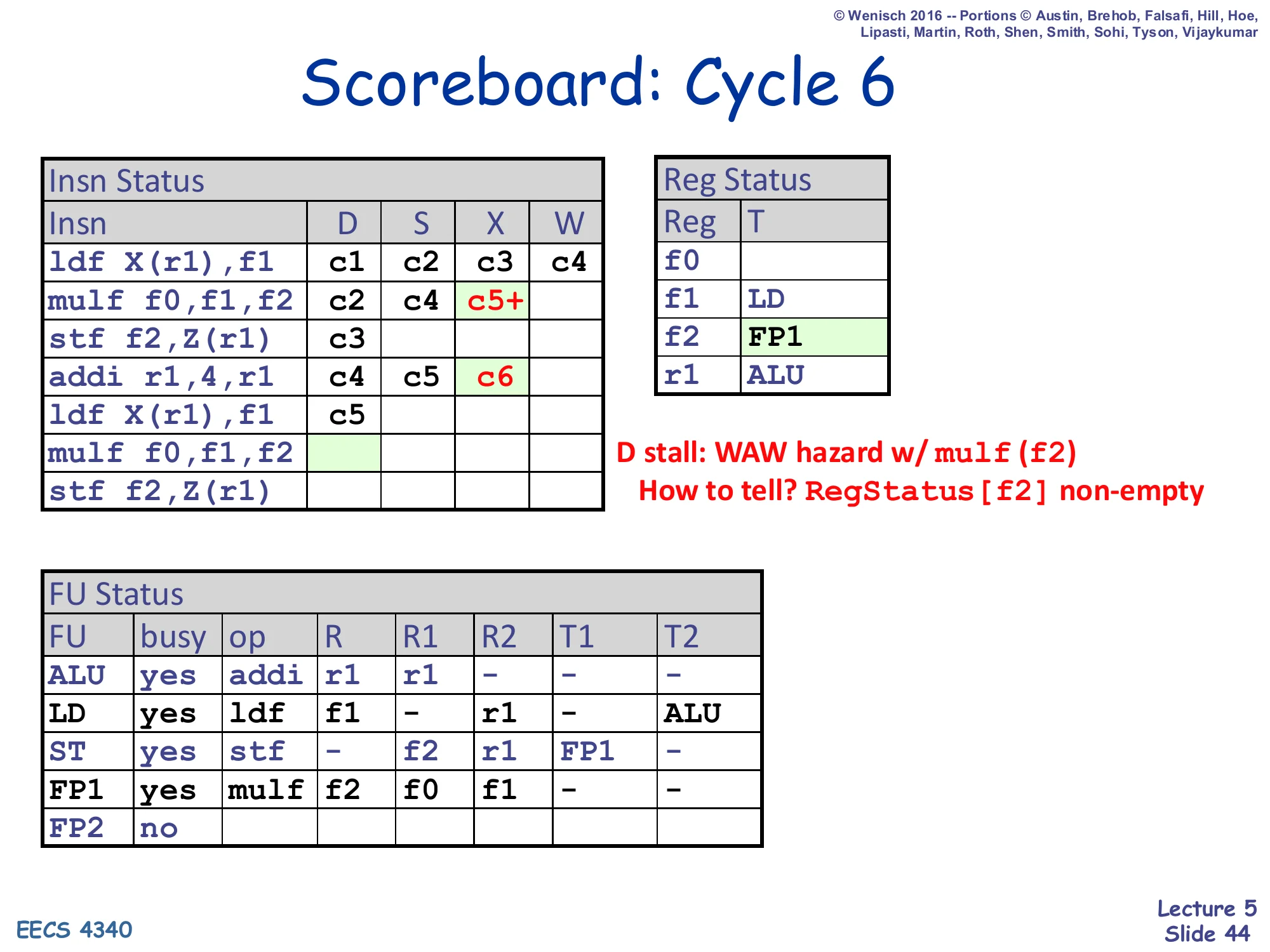
Insn Status — ldf₁: c1,c2,c3,c4; mulf₁: c2,c4,c5+ (still executing); stf₁: D=c3; addi: c4,c5,X=c6; ldf₂: D=c5; mulf₂ (second iteration): D stalled (highlighted blank cell)

Reg Status — f1: LD; f2: FP1; r1: ALU

FU Status — ALU executing addi; LD waiting (T2=ALU); ST waiting on FP1; FP1 busy with mulf₁ (multi-cycle); FP2: free

D stall: WAW hazard w/ mulf (f2). How to tell? RegStatus[f2] non-empty.

Cycle 6 illustrates the scoreboard’s painful WAW limitation. The second iteration’s mulf f0,f1,f2 tries to dispatch — FP2 is free, no structural conflict — but Reg Status[f2] is non-empty (it still holds FP1, because the first mulf has not yet written f2). That is a WAW hazard: dispatching mulf₂ would set Reg Status[f2] = FP2, but then if mulf₁ wrote after mulf₂ the architectural f2 would hold the wrong (older) value. So D stalls, and because dispatch is in-order this stall back-propagates and prevents the seventh instruction from entering as well. This is exactly the scheduling cliff described on slide 51 (“limited scheduling scope: structural/WAW hazards delay dispatch”). With renaming (Tomasulo), this WAW would simply produce a fresh physical register and dispatch would proceed.

Scoreboard: Cycle 7

Show slide text

Scoreboard: Cycle 7

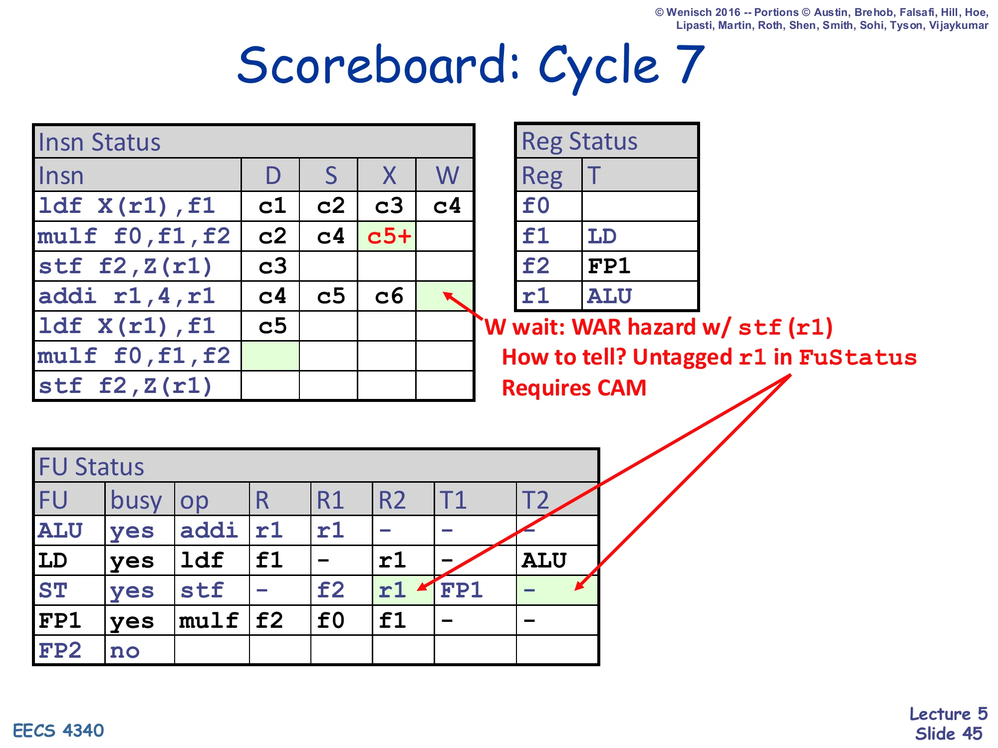
Insn Status — addi: c4, c5, c6 with W stalled (highlighted); mulf₁: still executing (c5+); ldf₂: D=c5

Annotation: W wait: WAR hazard w/ stf (r1). How to tell? Untagged r1 in FuStatus. Requires CAM.

FU Status — ALU has addi (R=r1, R1=r1) finished executing; LD waiting (T2=ALU still); ST has stf (R1=f2, R2=r1, T1=FP1, T2=–) — note T2 is clear meaning stf already read r1 and is sitting in execute; FP1 busy executing mulf₁

Cycle 7 demonstrates the WAR-hazard delay at writeback. The addi has finished execute and wants to write r1, but the older stf has read r1 (its T2 is clear, meaning the issued stf is sitting in the ST FU with the old r1 value already latched at issue). Writing r1 now would be safe in fact — stf already has the value — but the scoreboard cannot tell that the read has completed; it can only tell that the older instruction had r1 as a source operand. The WAR check is implemented as a CAM scan: “is there any FU entry whose source register name (untagged) equals my destination register?” The CAM-search annotation is honest about the cost: every writeback potentially scans every source field of every FU entry to detect this WAR. The addi will have to wait until stf retires (issues out of S) before it can write r1.

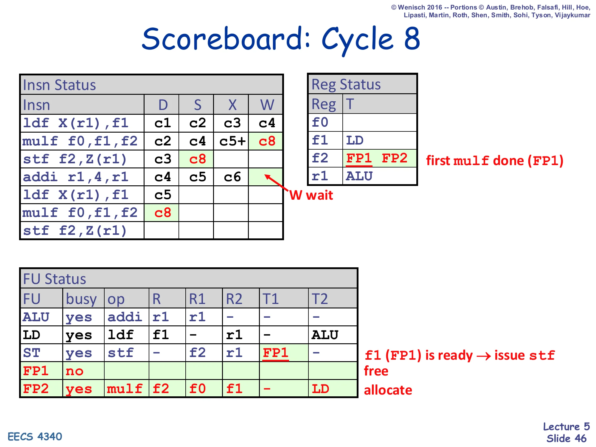
Scoreboard: Cycle 8

Show slide text

Scoreboard: Cycle 8

Insn Status — mulf₁: c2, c4, c5+, W=c8; stf₁: D=c3, S=c8; addi: c4, c5, c6, W still waiting; mulf₂: D=c8 now succeeds

Reg Status — f2: ~~FP1~~ FP2 (FP1 just freed by mulf₁ writeback, then FP2 newly allocated by mulf₂)

FU Status — FP1: free; FP2: yes, mulf, R=f2, R1=f0, R2=f1, T2=LD; ST broadcast clears stf.T1 (f1 ready) — first mulf done (FP1); f1 (FP1) is ready → issue stf — free, allocate

Cycle 8 is dense: mulf₁ writes back (W = c8 — the 3-cycle FP add latency means the multi-cycle X starting in c5 finishes in c7 and writeback happens in c8 with the ready check). Three things flow from that single writeback: (1) FP1’s tag is broadcast and clears the stf’s T1 (which was waiting on FP1.f2 → clear means stf’s f2 source is ready and stf can issue now: S = c8). (2) Reg Status[f2] is cleared, which removes the WAW hazard that had been blocking mulf₂ — so mulf₂ finally dispatches at c8 (D = c8) and is allocated FP2. (3) FP1 is freed, and Reg Status[f2] is re-set to FP2 (the new producer). Notice however that addi still cannot write back: the WAR with the older stf-on-r1 is still pending.

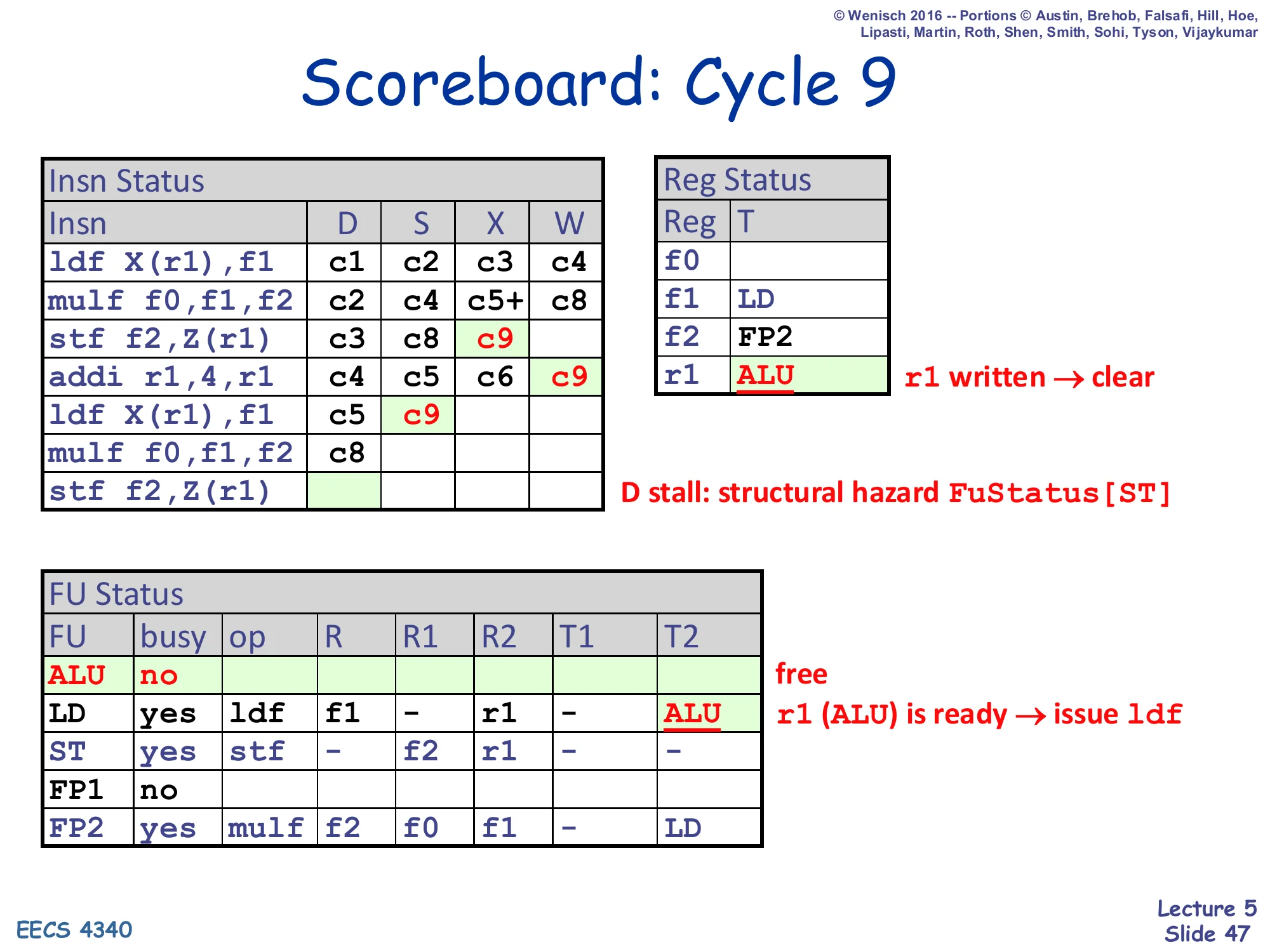
Scoreboard: Cycle 9

Show slide text

Scoreboard: Cycle 9

Insn Status — stf₁: D=c3, S=c8, X=c9; addi: c4, c5, c6, W=c9; ldf₂: D=c5, S=c9; mulf₂: D=c8; stf₂: D stalled (structural hazard FuStatus[ST])

Reg Status — r1: ~~ALU~~ (cleared, addi wrote r1)

FU Status — ALU: free; LD: ldf (T2=ALU still showing — but that broadcast just cleared LD.T2 → ldf₂ issues this cycle)

Cycle 9: addi finally writes back (W = c9) because the older stf has now issued (S = c8) — the WAR is resolved. The addi’s tag broadcast clears LD.T2 (which had been waiting on ALU = addi), so ldf₂ issues immediately the same cycle (S = c9). Reg Status[r1] is cleared. ALU is freed. Meanwhile stf₂ tries to dispatch but the ST unit is still busy with stf₁ (which is in execute) — that is a structural hazard and stf₂ stalls in D. This is the second iteration’s first dispatch stall, again caused by the scoreboard’s tight 1-entry-per-FU model. Two more cycles of cascading W/S/D events are ahead before the schedule converges.

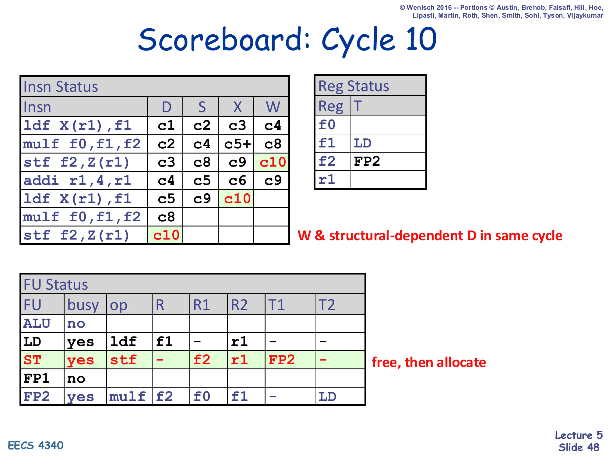
Scoreboard: Cycle 10

Show slide text

Scoreboard: Cycle 10

Insn Status — stf₁: c3, c8, c9, W=c10; ldf₂: c5, c9, X=c10; stf₂: D=c10 (now succeeds)

Reg Status — r1: cleared (also via stf, no — only addi wrote r1)

FU Status — ST: free, then re-allocated to stf₂ (free, then allocate); LD: ldf₂ executing; FP2: mulf₂ still waiting (T2=LD pending)

Annotation: W & structural-dependent D in same cycle

Cycle 10 illustrates the second “in-same-cycle” bypass concession from the rules slide: stf₁ writes back and frees the ST FU; in the same cycle stf₂ — which had been blocked on D last cycle by exactly that structural hazard — dispatches into the now-free ST entry. Without this concession stf₂ would lose another cycle. The scoreboard schedule for this snippet now stretches from c1 to c17 (according to the comparison table on slide 49). The remaining cycles (11–17) repeat the same pattern: ldf₂ writes back, mulf₂ issues, stf₂ waits on mulf₂, etc. The lecture stops drawing further individual cycles because the algorithm is now fully demonstrated.

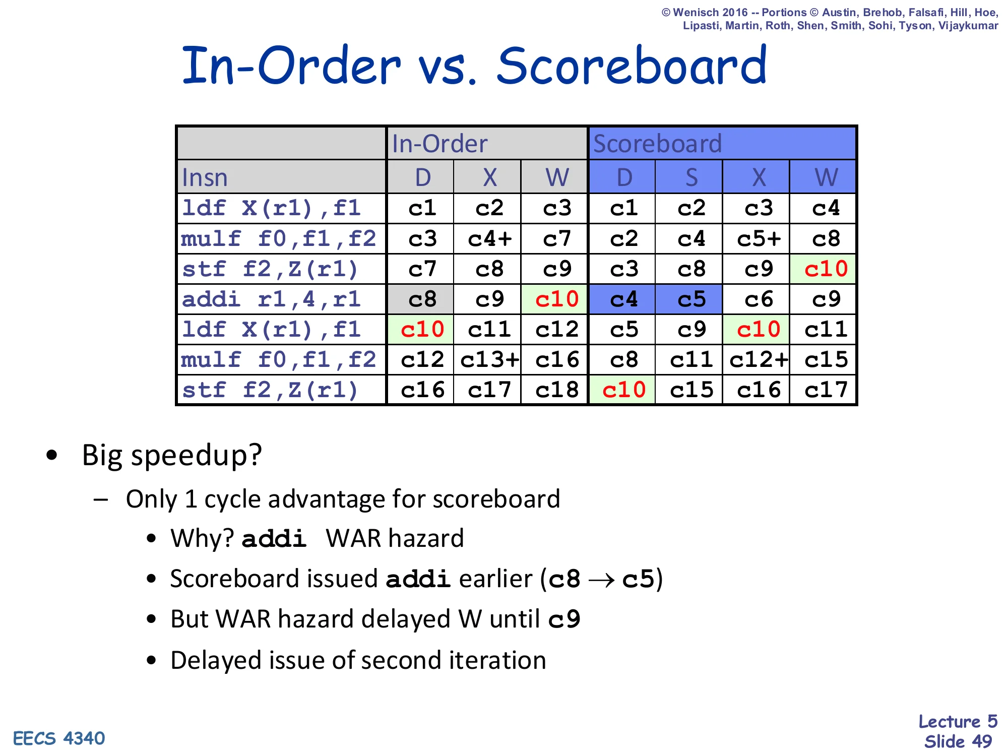
In-Order vs. Scoreboard

Show slide text

In-Order vs. Scoreboard

Insn	In-Order D	X	W	Scoreboard D	S	X	W
`ldf X(r1),f1`	c1	c2	c3	c1	c2	c3	c4
`mulf f0,f1,f2`	c3	c4+	c7	c2	c4	c5+	c8
`stf f2,Z(r1)`	c7	c8	c9	c3	c8	c9	c10
`addi r1,4,r1`	c8	c9	c10	c4	c5	c6	c9
`ldf X(r1),f1`	c10	c11	c12	c5	c9	c10	c11
`mulf f0,f1,f2`	c12	c13+	c16	c8	c11	c12+	c15
`stf f2,Z(r1)`	c16	c17	c18	c10	c15	c16	c17

Big speedup?
- Only 1 cycle advantage for scoreboard
- Why? addi WAR hazard
- Scoreboard issued addi earlier (c8 → c5)
- But WAR hazard delayed W until c9
- Delayed issue of second iteration

This is the scoreboard’s reality check. Compared head-to-head against the in-order baseline (slide 23), the scoreboard executes the same seven-instruction snippet in 17 cycles instead of 18 — a 1-cycle improvement. The reason is sobering: the scoreboard did aggressively issue addi ahead of stf (c5 vs c8 in-order), but the WAR hazard between addi and the older stf forced the addi’s W back to c9. That delay then chained to delay the second-iteration ldf₂’s R1=ALU clearing to c9, which delayed mulf₂’s issue to c11, etc. The scoreboard’s central problem is that it is fast at issue but slow at writeback whenever there is a WAR. This is exactly what register renaming (Tomasulo) fixes: by giving the addi a fresh physical name, there is no architectural WAR with the older stf, and the writeback can happen as soon as execute finishes.

In-Order vs. Scoreboard II: Cache Miss

Show slide text

In-Order vs. Scoreboard II: Cache Miss

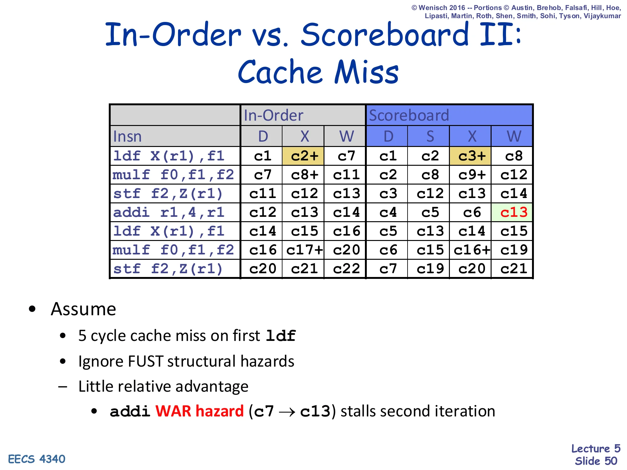
Insn	In-Order D	X	W	Scoreboard D	S	X	W
`ldf X(r1),f1`	c1	c2+	c7	c1	c2	c3+	c8
`mulf f0,f1,f2`	c7	c8+	c11	c2	c8	c9+	c12
`stf f2,Z(r1)`	c11	c12	c13	c3	c12	c13	c14
`addi r1,4,r1`	c12	c13	c14	c4	c5	c6	c13
`ldf X(r1),f1`	c14	c15	c16	c5	c13	c14	c15
`mulf f0,f1,f2`	c16	c17+	c20	c6	c15	c16+	c19
`stf f2,Z(r1)`	c20	c21	c22	c7	c19	c20	c21

Assume
- 5 cycle cache miss on first ldf
- Ignore FUST structural hazards
- Little relative advantage
  - addi WAR hazard (c7 → c13) stalls second iteration

When the first ldf takes a 5-cycle cache miss, both schemes pay the latency, but the scoreboard’s relative gain shrinks again because of the same WAR disease. The scoreboard issues addi at c5 and finishes execute at c6, but Reg Status[r1] cannot be cleared until the older stf retires r1 — which now happens around c13 because the long cache miss pushed everything downstream. So addi’s W is stalled from c6 → c13, and the second-iteration ldf (which depends on the new r1) cannot issue until c13. Result: scoreboard finishes the snippet in 21 cycles vs in-order’s 22, again essentially a one-cycle improvement. The lesson is that the scoreboard’s win is bottlenecked by its own WAW/WAR pessimism — long-latency events expose this even more sharply. Tomasulo will close this gap.

Scoreboard Redux

Show slide text

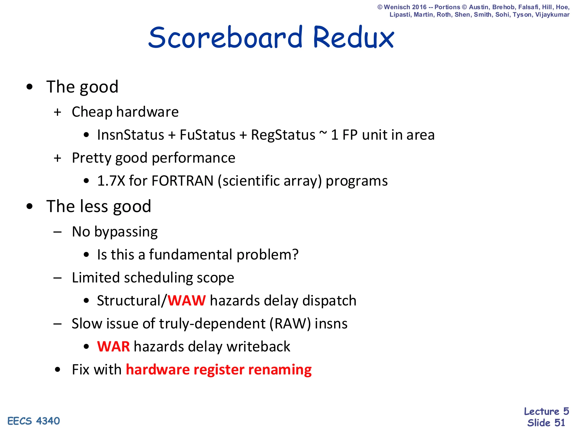
Scoreboard Redux

The good
- $+$ $+$ Cheap hardware
  - InsnStatus + FuStatus + RegStatus ~ 1 FP unit in area
- $+$ $+$ Pretty good performance
  - 1.7× for FORTRAN (scientific array) programs
The less good
- $-$ No bypassing — Is this a fundamental problem?
- $-$ $-$ Limited scheduling scope
  - Structural/WAW hazards delay dispatch
- $-$ $-$ Slow issue of truly-dependent (RAW) insns
  - WAR hazards delay writeback
Fix with hardware register renaming

The retrospective on scoreboarding. The good: it is genuinely cheap (the three tracking tables together are about the area of one FP unit — astonishing for the era), and on FORTRAN-style scientific code (lots of independent FP work, few control hazards) it delivered a 1.7× speedup over a comparable in-order machine. The less good: no bypassing means even back-to-back RAW pairs eat the full produce/consume latency; structural hazards on the FUST entries and WAW hazards on Reg Status both stall the in-order dispatch and back-propagate to younger instructions; and WAR hazards stall writeback even when the execute has finished. The summary diagnosis at the bottom — “fix with hardware register renaming” — is the bridge to the next lecture: Tomasulo introduces reservation-station-based renaming and a common data bus that together fix all three pain points.

Readings

Show slide text

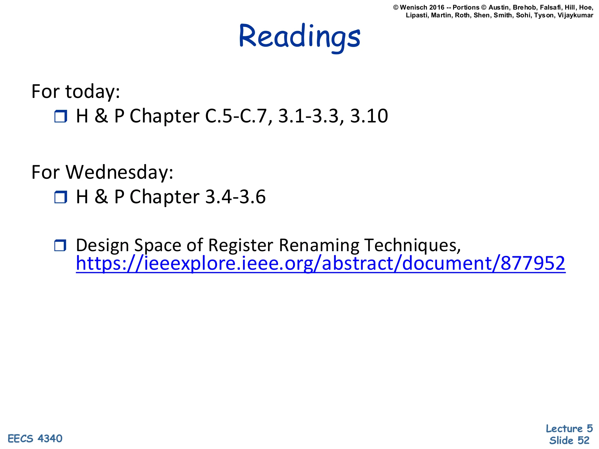
Readings

For today:

H & P Chapter C.5–C.7, 3.1–3.3, 3.10

For Wednesday:

H & P Chapter 3.4–3.6
Design Space of Register Renaming Techniques, https://ieeexplore.ieee.org/abstract/document/877952

Announcements

Show slide text

Announcements

No lab this Wednesday
- We will have a lecture instead
Project #3
- Due: 25-Feb-26

https://courseworks2.columbia.edu/courses/237081